An important component in the cost of doing business is the inventory cost associated with work in process (WIP). This is composed of partially completed products either undergoing or awaiting processing. For many companies, WIP is a large component of the total assets of the company. Compared to other assets of the company, WIP in almost all cases does not contribute to profitability, and it is often a goal of management to reduce or eliminate it. The popular just-in-time (JIT) manufacturing philosophy has the goal of producing a unit of product only as it is required, thus reducing WIP to its absolute minimum. Along with this we have JIT raw material deliveries and JIT finished goods manufacturing, all designed to reduce as much as possible the level of inventory.

The time a product takes to pass through the manufacturing process, or the cycle time, is strongly related to the WIP. There are many reasons we would like to keep this time small rather than large, so the reduction of WIP has the dual effect of reducing cycle time.

WIP does have the positive function of protection against variability. One reason for providing finished goods inventory is to protect against the variability of customer demand. A reason for keeping raw material inventory is to protect against the uncertainty of raw material supply. WIP within the process protects against machine operation time variability and flow variability. It is important to keep a buffer stock available for a critical machine so that the machine is never starved for materials. WIP may protect against machine failures by allowing some parts of the process to operate while others are down for repair.

WIP is also used to reduce the effects of setup times (or costs). A product with a large setup time on a machine must be produced in large lots so that the setup time is spread over a number of units. Raw materials are often ordered in large lots because transportation and ordering costs have economies of scale and large fixed costs cause small lots to be expensive. We will see that large lot sizes increase WIP.

The add-in provides a variety of models for measuring WIP, cycle time and the cost of WIP. Each model describes a component of the production system. The results can be combined to evaluate an entire system. We assume steady-state flows with continuous and constant demands. Except for the queuing model, we assume no random variability. Although time the spent on a machine is computed, no scheduling of several products that may be using the same machine is considered. The models are simple and deterministic, but they do provide insights on the aspects of the system that contribute the most to WIP and its cost.

To create a model choose Add Inventory from the menu. The dialog below is presented. Near the top of the dialog we see the address of the cell where the top of the component definition will be placed. The Name entered here is used for naming ranges. The Time Interval defines the interval used for all rates and time intervals. The Replications box allows several components to be simultaneously created. Along the left margin the component models are listed. The top button identifies the storage inventory that has previously been described. Except for the last, the remainder identify WIP component models. We choose the Lot Change model for the first example. The remainder of the dialog options are not used for WIP models.

The Params button presents a new dialog, illustrated below. The dialog allows direct entry of the parameters associated with the WIP model. Parameters entered with this dialog are placed on the Excel worksheet. They may be changed arbitrarily once the model is created, so it is really unnecessary to set the parameters here.

The Display button on the Inventory definition dialog is not used for the WIP models.

On the remainder of this page, we consider the several models that are available and explain the meaning of the parameters and results for each model.

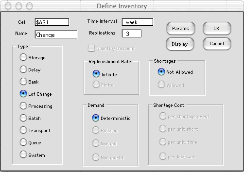
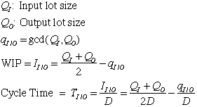
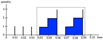
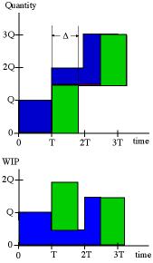
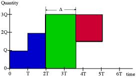
Lot sizes play an important role in the models. Throughout we assume that lots travel through the system uniformly in time. With a flow rate of 100 per week and a lot size of 1, a unit passes any given point in the system every 0.01 weeks. With a lot size of 3, a lot of three units passes the point every 0.03 weeks. The figure below shows the process involved with changing lot sizes from 1 to 3. The lot size change occurs at an accumulation point where single units enter the point every 0.01 weeks and lots of 3 leave every 0.03 weeks. The figure shows an accumulation beginning at time 0.04. Units accumulate at 0.05 and 0.06. At time 0.06 the lot of 3 units has accumulated and is released. The inventory pattern is periodic. A second period is shown beginning at time 0.07. Steady state will see the pattern below repeated every 0.03 weeks.

The blue area indicates WIP that accumulates because of the lot size change. Considering a period of 0.03 weeks, the area under the WIP curve is 3 units. The average WIP is

WIP = Area for one period/Length of period

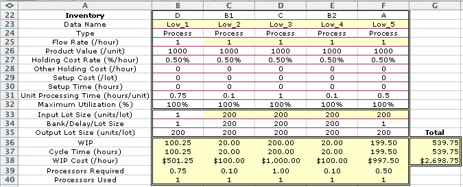
For the example the average WIP is 1. The average residence time for a unit experiencing a lot size change is determined by Little's Law. To agree with common terminology used when discussing manufacturing systems we call the average residence time the cycle time.

Cycle Time = WIP/Flow rate

For the example the flow rate is 100/week, therefore the cycle time for the lot size change operation is 0.01 weeks. Note that the use of cycle time may result in some confusion since we have previously used the term to describe the interval over which the inventory pattern repeats. In this discussion we call the repeating interval the period.

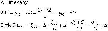
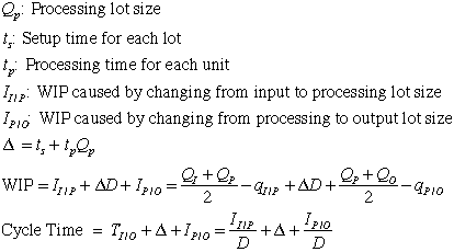
To understand the lot size change operation, consider the figures below. The figure shows the cumulative arrivals and departures during a change of lot size from Q to 1.5Q. The cumulative arrivals are shown in blue. The cumulative departures are in red overlaying the arrivals. The length of the period is 3T, where T = Q/D.

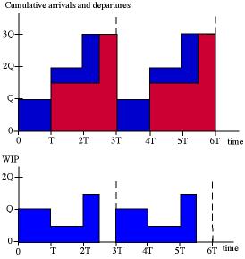
For feasibility the departures can occur only after arrivals, so we have shifted the departure graph so that it never exceeds the arrival graph. The two touch at time T, so T is the minimum feasible time shift. Two cycles of the resultant WIP are shown in the second figure. This figure is constructed by subtracting the departure graph from the arrival graph. 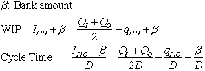To compute the average WIP and the resultant cycle time we use the simple formulas below.

The WIP is the average of the input and output lot sizes, less their greatest common divisor. For the example, Q is the greatest common divisor, so

WIP = 1.25Q - Q = 0.25Q

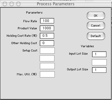
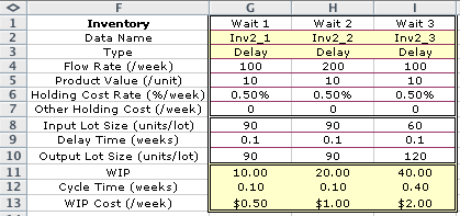
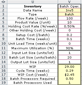
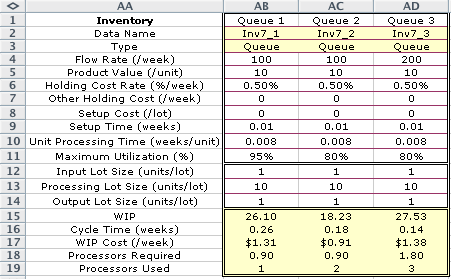
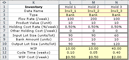
The figure below shows the entries placed on the worksheet by the add-in for the lot size change component. Although the display can appear anywhere on the worksheet the example is placed in the cells to the right and below cell A1. The titles are in column A and the data and results are in column B, C and D.

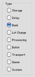
The first part of the display holds the parameters of the model. The number of rows used depends on the type of model. For the example the parameters are in rows 1 through 7. The first entry is set by the user to identify the inventory. The other parameters may be changed except the Data Name and Type. The data name is used to name cells on the worksheet. The type is used by the program and should not be changed. All numeric parameters are to be nonnegative.

Rows 8 and 9 hold the instance variables. The important variables for the lot size change component is the input and output lot sizes. We give different values for three cases.

The next three rows, row 10 through row 12, hold the instance results. The WIP is the average inventory produced by this component. The Cycle Time is the average residence time that an item remains in inventory. Finally, the WIP Cost is the cost associated with holding the average WIP. Since the value of a unit of WIP is $1000 and the holding cost rate is 0.5% per week, the holding cost is $5 per unit per week.

We see in the illustration, that when there is no change in lot size, there is no WIP. Changing the lot size from 1 to 3 results in the WIP and cycle time previously described. The change from 3 to 1 is symmetric to the change from 1 to 3 and has the same WIP.

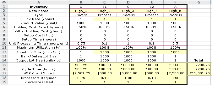
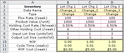
A second example is shown below. Here we hold the average of the input and output lot sizes at 90, but change their relative values.

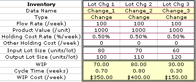
The results are perhaps counterintuitive. When the input and output lot sizes have the greatest difference in case 3, the WIP is the smallest. Since all three cases have the same average, 90, we note the major effect of the gdc. If the lot sizes are the same, the gdc is the same as the lot size, so the WIP is 0. When the lot sizes differ by a factor of 2, the gdc is the smaller of the two lot sizes, and the WIP is the average less the smaller lot size (90 - 60 = 30 as in the third case). The effect of a lot size change on WIP is highly nonlinear. Note that the WIP caused by a lot size change is a function of only the input and output lot sizes and not on the flow rate.

There are many causes for delays in manufacturing systems. Sometimes delays are part of the manufacturing process such as a drying period required after painting. Others are due to undesirable occurrences such as part shortages or scheduling conflicts. In every case we model a delay as a fixed time, independent of flow rate, added to the cycle time of a lot size change. The illustration shows a delay of 0.1 weeks. The resultant WIP is determined by Little's Law. The first two cases are the same except that the flow rate for Wait 2 is twice that of Wait 1. With the delay constant, the WIP is doubled. Wait 3 shows the result combining a lot size change with the delay. The lot size change contributes 30 to the WIP while the delay contributes 10.

The figure on the left illustrates the effect of the delay. Note that the delay is in addition to the time shift caused by the lot size change.

A bank is an inventory of constant size. The purpose for the Bank or buffer is usually to provide protection against some unwanted disturbance. Although we do not model the variability that gives rise to banks, we can measure the effect on WIP and cycle time. The example below shows the results for a bank of size 10. For the first case, Hold 1, the bank is fixed at 10 and there is no lot size change. A straight forward application of Little's Law result in a mean cycle time of 0.1 weeks.

The second case illustrates that a doubling of the flow rate results a halving of the cycle time. This is necessary since the amount of WIP is held constant. In the third case we illustrate the effect of a lot size change. The resultant WIP adds to the bank.

The back adds directly to the WIP due to the lot size change.

The process component models an operation within a manufacturing process. Items enter the operation periodically in number equal to the input lot size. The items are grouped in number equal to the processing lot size. Each lot requires a processing time equal to setup time plus the unit processing time multiplied by the processing lot size. The output of the operation is gathered into lots equal in number to the output lot size and pass from the operation.

The data segment of the display has four new entries:

• the setup cost is expended each time a lot is processed
• the setup time measures the time required for setup each time a single lot is begun
• the unit processing time is expended for each member of the lot
• the maximum utilization is the proportion of the time that can be used on the machine that performs the operation.

The instance variables are the input, processing and output lot sizes. The instance results have five entries:

• the WIP is the average number of items resident in the operation
• the cycle time is the average time an item remains in the process including the time to change lot sizes
• the WIP cost includes the cost of the opportunity cost of the WIP that represents the holding cost and also the weekly cost associated with setups
• the processors required is based on the total time the processors implementing the operation
• the processors used is the integer number of machines necessary when each machine can operated only up to the maximum utilization

In the first case, the WIP required to first change the lot size from 1 to 10 and then from 1 back to 10 is 19. The WIP added by the processing time is 9, for a total WIP of 18. In the second case a larger lot size is used. This increases the WIP because each lot requires more time. It decreases the cost because larger processing lots require fewer setups. The third case has input and output lot sizes equal to the processing lot size. This reduces the time required for lot changes. Note that we have reduced the maximum utilization to 80%. Although the processors required remain an 0.9 the number of processors used must be increased to 2.

The figure illustrates the cumulative inputs and outputs over a cycle. The input lot size is Q, the processing lot size is 3Q, and the output lot size is 2Q. The blue area is WIP that has arrived, but is gathering to obtain a processing lot. The green area represents time in processing. The red area is WIP waiting to leave the operation.

The equations computing WIP and cycle time for a processing operation are as below.

The batch operation is similar to the processing operation except usually the fixed time is considerably greater than the unit processing time. A typical batch process is a firing furnace in ceramic manufacture. A number of items, the batch, is placed in the furnace and heated for a specified time. All the items remain in the furnace for the required time. The load time is the time expended for each unit.

The parameters and instance variables are the same as for the process component except some have been titled more appropriately for the batch process.

The transport operation is similar to the batch operation. Again the fixed time representing the time for transporting a load of items is the primary time. The variable time represents the time required to load and unload each item.

The parameters and instance variables are the same as for the process component except some have been titled more appropriately for the transport component.

Although we have neglected statistical variability in our models, the queuing model provides an estimate of the effect of variability in arrival and service times.

The parameters and instance variables are the same as for the process component. To compute the WIP associated with the queuing station we use the formulas from queuing analysis. In particular we use the approximation formulas for the non-Markovian system. Because the queue processes items in lots, the processing times for lots is assumed to have an Erlang distribution. Also the times between arrival are assumed to come from an Erlang distribution. The number of service channels for a station is governed by the total processing time required and the maximum utilization of the channels.

The system option constructs a model of several components arranged in series and adds the results. An example is shown below. Here we consider a sequence of processing operations. We are comparing the WIP and total cycle time for high and low lot sizes. From observing the two results we see that the smaller lot size results in a total WIP and cycle time less than 1/4 the value for the larger lot size.

The components of the system can be any of those considered on this page. They are identified by the word placed in the Type row. Note that we have not colored the cells yellow for this display. The delay, bank and lot size components use fewer parameters than than the other components. The contents of the extra cells are ignored.

The flow rates in row 4 are all linked by formulas to the flow rate of the first component. All flows are equal for this series arrangement. The System command on the menu allows several other arrangements of components including a tree arrangement and a general network arrangement. These options are described on the next page.

Lot size 1000