Welcome to the
SolverTable add-in (version 2007.2)
This add-in is a natural extension to the Solver add-in incorporated in Excel. SolverTable performs sensitivity analysis for an Excel optimization model, and, in most cases, its output is more relevant and understandable than the optional sensitivity output provided by Solver itself. (Besides, we have learned that Microsoft “broke” something in Excel 2007, so that Solver’s Sensitivity Report might not be available!)
SolverTable is very easy to use, as I describe below. All it requires is an existing optimization model. That is, there must be a spreadsheet model already built, and the corresponding Solver dialog box must already have been filled in. This document explains how to use SolverTable, and it illustrates the procedure with several screen shots. Note: This version of SolverTable has been developed to work with Excel 2007 (aka Excel 12). You will see only minor differences (in the user interface) from the previous version of SolverTable. This version will not work with previous versions of Excel.
Sections of this
Help file
- Loading SolverTable
- Unloading SolverTable
- An example file
- Running SolverTable
- SolverTable Difficulties
- Other Notes
Loading
SolverTable
To load SolverTable, proceed as follows:
1) Copy the SolverTable.xlam file and the corresponding help files (SolverTableHelp.htm and the various SolverTable .gif files) to a common folder on your hard drive. I recommend creating a SolverTable folder for this purpose under Microsoft’s Library folder, i.e., c:\Program Files\Microsoft Office\Office12\Library\SolverTable, because this folder is in Microsoft’s “trusted” list. If you want to store the files somewhere else, e.g., D:\SolverTable, then you should add this folder to the trusted list. (To do so, Click on the Office button, then Excel Options, then Trust Center, then Trust Center Settings, then Trusted Locations, and then Add new location.)
2) (One-time only step) Because of the way Solver works and the way SolverTable invokes Solver, you need to change a macro security setting on your PC. Make sure the Developer tab is visible. (If it isn’t, click on the Office button and then Excel Options. In the Popular group, check the Show Developer tab in the Ribbon option.) On the Developer ribbon, click on Macro Security and make sure the “Trust access to the VBA project object model” option is checked. (As long as you’re there, I recommend that you check the second option in the top group: “Disable all macros with notification.”)
3) In Excel, load SolverTable into memory. There are two ways to do this. Regardless of the way you use, you will know that SolverTable is loaded when you see a SolverTable item on the Add-Ins ribbon.
a) Open the SolverTable.xlam file directly by double-clicking on it in Windows Explorer. If this file is buried way down in some folder, this way might not be very convenient, but you can accomplish the same thing by putting a shortcut to this file on your desktop, so that it’s just one click away. The advantage (or disadvantage?) of this method is that if you then close Excel and reopen it, SolverTable won’t be loaded; you’ll have to load it again.
b) Click on the Office button, then on Excel Options, then on Add-Ins, and then on the Go button at the bottom. Here you see the familiar Add-ins dialog box from earlier versions of Excel. If this is your first time to load SolverTable, you will need to click on the Browse button to find the SolverTable.xlam file. Otherwise, there should be a SolverTable item in the list of available add-ins. Just check its box, and click on OK. The advantage of this second method is that if you then close Excel and reopen it, SolverTable will open automatically. In fact, it will keep opening until you uncheck SolverTable on the Add-Ins list.
Note: In previous versions of SolverTable, there were two add-in files, SolverTable and SolverTable1. The current version simplifies this, so that there is now only SolverTable.xlam.
Unloading
SolverTable
To unload this add-in (remove it from memory), just close Excel (if you used method a) above), or uncheck the SolverTable box in the Add-ins list (if you used method b) above).
An example file
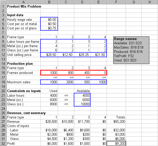
To illustrate SolverTable, I will use the standard product mix model, a version of which appears in Figure 1. (The conventions I use are that the inputs are in blue borders, the changing cells are in red borders, and the objective cell is in a black border, but you can use any conventions you like.) I assume the Solver dialog box has already been completed in the obvious way (including checks in the Linear and Non-Negative boxes). Actually, this model has already been optimized, but this is not necessary for running SolverTable.
Figure 1
Running
SolverTable
The purpose of SolverTable is very much like that of an Excel data table: to vary one or two inputs and keep track of one or more outputs. The main difference is that SolverTable runs Solver for each input value (or combination of input values) and reports the optimal results in the table. Like data tables, there are essentially two options: oneway tables and twoway tables, depending on whether there are one or two input cells. However, unlike Excel data tables, there can be multiple output cells for oneway and twoway tables. In the latter case, SolverTable creates a separate table for each output cell. Note that a table created by SolverTable retains no links to the original data. If you want to change anything about the table, you must rerun SolverTable.
Creating
a oneway table
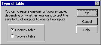
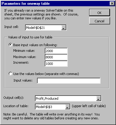
To illustrate a oneway table, I will see how the optimal profit and the optimal product mix (changing cells) vary as the number of labor hours available (cell D21) varies from 2000 to 8000 in increments of 1000. Begin by selecting the Run SolverTable item from the SolverTable dropdown on the Add-Ins ribbon. You will first be asked whether you have a Solver model on this sheet. For this example, you should say Yes. But if you inadvertently ran SolverTable on a sheet without a Solver model, this would give you a way to back out gracefully. You then see the dialog box in Figure 2. Fill it out as shown and click on OK.
Figure 2
The next dialog box, shown in Figure 3, requires you to specify the input cell, the input values (which are assumed to be in regular increments if you choose the first option, or any list of values if you choose the second option), the output cells, and a location for the table. Note that range names can be used if they exist. SolverTable checks your entries in this dialog box for "obvious" errors. For example, the input cell should not contain a formula or a label, the output range should not contain the input cell, the table location should not write over existing values (unless you say it is OK to do so), and so on. However, I cannot guarantee that it checks for everything, so be careful when you make these entries. Be especially careful that you choose a location for the table that does not write over any information you don't want to lose (even though you will be warned if you try to do so).
Figure 3
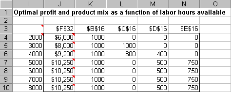
The table itself appears in Figure 4. (I have added the heading in row 1 manually.) The small red triangles are Excel comments that SolverTable automatically adds to a number of cells. For example, the comment in cell I4 reminds you what the input cell is (in this case, D21). The comments in column J are the Solver messages you normally see after running Solver. For this example, they all contain the message you hope to see: "Solver found a solution. All constraints and optimality conditions are satisfied." However, if there is no feasible solution, say, then the comment will alert you to this. Note that unlike an Excel data table, SolverTable does not put formulas at the top of the table (in row 3 of the figure), because this wouldn't make sense. However, it does put the cell addresses of the output cells. This way, you can remember which outputs are being reported.
Figure 4
Creating
a twoway table
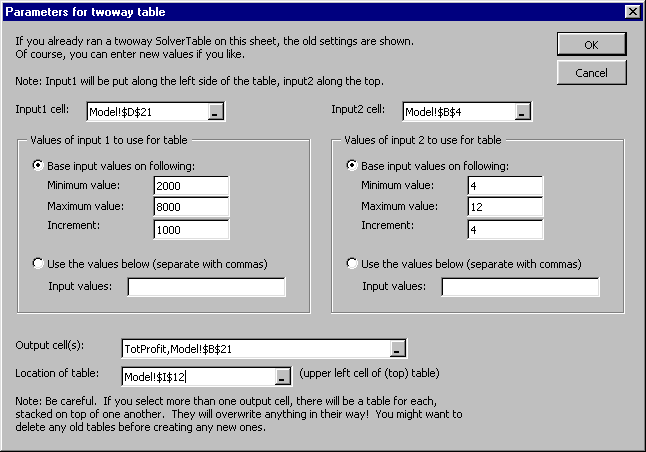
To create a twoway table, go through the same steps as above for a oneway table, but check the twoway option in Figure 2. Then the twoway dialog box in Figure 5 appears. Here, I'll assume that both labor hour availability (D21) and hourly wage rate (B4) are being varied, and that the desired outputs are the optimal profit and the number of labor hours used (B21). (Any output cells could be selected.)
Figure 5
SolverTable then creates as many tables as there are output cells (in a vertical direction), as shown in Figure 6. Note that each cell in a table corresponds to a Solver run. For example, when there are 4000 labor hours available and the wage rate is $4 per hour, the optimal profit is $25,200 (top table) and all 4000 labor hours are used (bottom table). Again, there are comments in selected cells. For example, the comments in cells I13 and J12 remind you that the input cells are D11 and B4. The comments in the body of each table report the Solver message, exactly as with oneway tables.
Figure 6
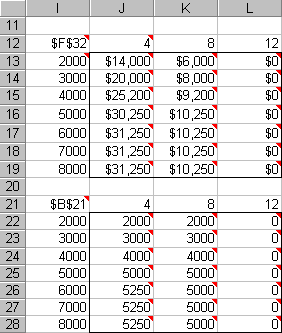
As with all Solver models, it is a good idea to take a close look at the answers and see whether they make sense. For example, column L in Figure 6 contains all zeroes. Does this make sense? Yes, it probably does. When the labor rate is $12 per hour and all other monetary inputs stay constant, labor is evidently too expensive for the company to make a profit. So it produces nothing!
Being
creative
With some imagination, you can get SolverTable to run some really interesting sensitivity analyses. For example, suppose you want to allow the availabilities of all three resources (labor, metal, and glass) to change by a common factor. Then you need to change the model slightly, as indicated in Figure 7. Now the original availabilities have been moved to column F, a change factor has been inserted in column H, and formulas have been entered for availabilities in column D. Specifically, the formula in cell D21 is =$H$21*F21, which is then copied down.
Figure 7

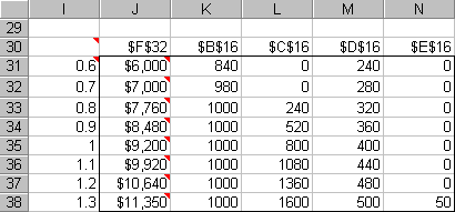
You can now do a oneway sensitivity analysis on this change factor, using the settings in Figure 8. The corresponding table appears in Figure 9.
Figure 8
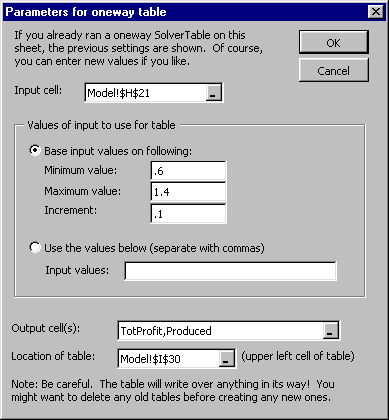
Figure 9
As another example, suppose you want to keep track of a function of several cells in the model. For example, suppose you want to keep track of the maximum number of frames of any single type produced, that is, the maximum of the changing cell values. You can't select this as an output directly because it doesn't appear anywhere in the model. But there is a simple solution: create a formula for it in some unused cell, and then specify this cell as an output cell.
SolverTable
Difficulties
SolverTable relies on Solver. In fact, SolverTable invokes Solver for each input value (or combination of input values). Therefore, any problems that people have experienced with Solver can occur with SolverTable. However, I have tried to overcome one of Solver's more annoying features: claiming that a model is not linear when you know it is linear. In case you have not run into this problem, I will describe it first. When your model is linear, you should check the Assume Linear Model box under Solver Options. This has two advantages. First, it uses a faster algorithm (the simplex method). Second, it is guaranteed (well, almost) to find the optimal solution if an optimal solution exists. However, Solver uses its own rules to check whether a model is linear. Because of numerical precision problems inherent in computers, Solver sometimes decides that a model is not linear, even though you know it is. In this case, it responds with an error message that the conditions for a linear model are not satisfied -- and it doesn't solve the problem.
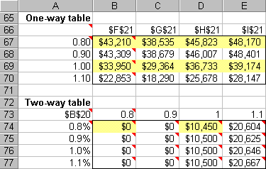
SolverTable automatically checks for this error message. If Solver gives it, then SolverTable reruns Solver with the Assume Linear Model box unchecked and reports the result. However, to let you know that all of this happened, the corresponding cells of the table are colored yellow, and the comments in these cells describe the situation. An example I encountered appears in Figure 10. This model is indeed linear. However, when I formed the oneway table, Solver thought the model was not linear for input values of 0.80 and 1.00, even though it agreed that it was linear for input values of 0.90 and 1.10. Similarly, for the twoway table, it thought the model was not linear for 2 of the 16 input combinations. This is clearly strange behavior, but it sometimes happens. (This was before Excel 2007. Maybe the Solver in Excel 2007 is different.) At least, SolverTable provides a solution (using a nonlinear algorithm) rather than the annoying "conditions for linear model are not satisfied" Solver message.
Figure 10
Other
Notes
- If you run a oneway SolverTable in a given workbook and
then run another, the settings dialog box (see Figure 3 or 8 above) show
the previous settings as a starting point. Of course, you can
change any or all of these. The same is true if you have run a twoway
SolverTable in a given workbook. (In case you're interested, these
settings are stored in a new worksheet called SolverTableSheet that is inserted into your workbook. However,
this worksheet is "very hidden" – you can't get to it
except by writing VBA code. If you really want to look at this hidden
sheet, or even delete it, you can do so, although it takes a bit of work.
First, press Alt-F11 to get to the Visual Basic Editor. On the left side
of the screen, in the Project Explorer, put your cursor on any of the
items in the file your Solver model is in. If you’ve run SolverTable
on it, you should see that one item in the file is the SolverTableSheet
worksheet. Now press Ctrl-G to open the Immediate Window, where you can
run single lines of VBA code. In the Immediate Window, type the line Worksheets(“SolverTableSheet”).Visible
= True and then press enter. Now the hidden sheet is no longer hidden,
and you can do anything you want with it.)
- As any programmer knows, it is practically impossible
to catch all of the bugs. The current version of SolverTable tries to
"trap" any error it encounters and present a message in a dialog
box that identifies the error. If you see one of these messages, please
report its information to me, so that I can see what error you encountered
as well as your version of Excel, Windows, and SolverTable (which all
appears in the dialog box).
Chris Albright, Kelley School of Business, Indiana University, albright@indiana.edu, October 2007