Statement

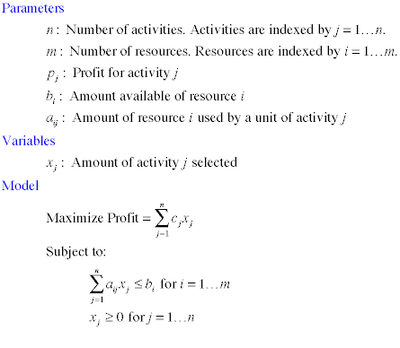
The type of problem most often identified with the application of linear program is the problem of distributing scarce resources among alternative activities. The Product Mix problem is a special case. In this example, we consider a manufacturing facility that produces five different products using four machines. The scarce resources are the times available on the machines and the alternative activities are the individual production volumes. The machine requirements in hours per unit are shown for each product in the table. With the exception of product 4 that does not require machine 1, each product must pass through all four machines. The unit profits are also shown in the table.

The facility has four machines of type 1, five of type 2, three of type 3 and seven of type 4. Each machine operates 40 hours per week. The problem is to determine the optimum weekly production quantities for the products. The goal is to maximize total profit. In constructing a model, the first step is to define the decision variables; the next step is to write the constraints and objective function in terms of these variables and the problem data. In the problem statement, phrases like "at least," "no greater than," "equal to," and "less than or equal to" imply one or more constraints.

Machine data and processing requirements (hrs./unit)

Model

Variable Definitions

Pj : quantity of product j produced, j = 1,...,5

Machine Availability Constraints

The number of hours available on each machine type is 40 times the number of machines. All the constraints are dimensioned in hours. For machine 1, for example, we have 40 hrs./machine ¥ 4 machines = 160 hrs.

Nonnegativity

Pj > 0 for j = 1,...,5

Objective Function

The unit profit coefficients are given in the table. Assuming proportionality, the profit maximization criterion can be written as:

 Maximize Z = 18P1+ 25P2 + 10P3 + 12P4 + 15P5

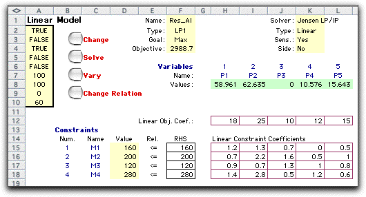
Solution

The model constructed with the Math Programming add-in is shown below. The model has been solved with the Jensen LP add-in. We note several things about the solution.

• The solution is not integer. Although practical considerations may demand that only integer quantities of the products be manufactured, the solution to a linear programming model is not, in general, integer. To obtain an optimum integer answer, one must specify in the model that the variables are to be integer. The resultant model is called an integer programming model and is much more difficult to solve for larger models. The analyst should report the optimal solution as shown, and then if necessary, round the solution to integer values. For this problem, rounding down the solution to: P1 = 59, P2 = 62, P3 = 0, P4 = 10 and P5 = 15 will result in a feasible solution, but the solution may not be optimal.
• The solution is basic. The simplex solution procedure used by the Jensen LP add-in will always return a basic solution. It will have as many basic variables as there are constraints. As described elsewhere in this site, basic variables are allowed to assume values that are not at their upper or lower bounds. Since there are four constraints in this problem, there are four basic variables, P1, P2, P4 and P5. Variable P3 and the slack variables for the constraints are the nonbasic variables.
• All the machine resources are bottlenecks for the optimum solution with the hours used exactly equal to the hours available. This is implied by the fact that the slack variables for the constraints are all zero.
• This model does not have lower or upper bounds specified for the variables. This is an option allowed with the Math Programming add-in. When not specified, lower bounds on variables are zero, and upper bounds are unlimited.

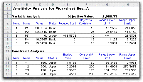
The sensitivity analysis amplifies the solution. The analysis shows the results of changing one parameter at a time. While a single parameter is changing, all other problem parameters are held constant. For changes in the limits of tight constraints, the values of the basic variables must also change so that the equations defining the solution remain satisfied.

Variable Analysis

• The "reduced cost" column indicates the increase in the objective function per unit change in the value of the associated variable. The reduced costs for the basic variables are all zero because the values of these variables are uniquely determined by the problem parameters and cannot be changed.
• The reduced cost of P3 indicates that if this variable were increased from 0 to 1 the objective value (or profit) will decrease by $13.53. It is not surprising that the reduced cost is negative since the optimum value of P3 is zero. When a nonbasic variable changes, the basic variables change so that the equations defining the solution remain satisfied. There is no information from the sensitivity analysis on how the basic variables change or how much P3 can change before the current basis becomes infeasible. Note that the reduced costs are really derivatives that indicate the rate of change. For degenerate solutions (where a basic variable is at one of its bounds) the amount a nonbasic variable may change before a basis change is required may actually be zero.
• The ranges at the right of the display indicate how far the associated objective coefficient may change before the current solution values (P1 through P5) must change to maintain optimality. For example, the unit profit on P1 may assume any value between 13.26 and 24.81. The "---" used for the lower limit of P3 indicates an indefinite lower bound. Since P3 is zero at the optimum, reducing its unit profit by any amount will make it even less appropriate to produce that product.

Constraint Analysis

• A shadow price indicates the increase in the objective value per unit increase of the associated constraint limit. The status of all the constraints are "Upper" indicating that the upper limits are tight. From the table we see that increasing the hour limit of 120 for M3 increases the objective value by the most ($8.96), while increasing the limit for M4 increases the objective value by the least ($0.36). Again, these quantities are rates of change. When the solution is degenerate, no change may actually be possible.
• The ranges at the right of the display indicate how far the limiting value may change while keeping the same optimum basis. The shadow prices remain valid within this range. As an example consider M1. For the solution, there are 160 hours of capacity for this machine. The capacity may range from 99.35 hours to 173 hours while keeping the same basis optimal. Changes above 120 cause an increase in profit of $4.82 per unit, while changes below 120 cause a reduction in profit by $4.82 per unit. As the value of one parameter changes, the other parameters remain constant and the basic variables change to keep the equations defining the solution satisfied.

General Resource Allocation Model

It is common to describe a problem class with a general algebraic model where numeric values are represented by lower case letters usually drawn from the early part of the alphabet. Variables are given alphabetical representations generally drawn from the later in the alphabet. Terms are combined with summation signs. The general resource allocation model is below. When the parameters are given specific numerical values the result is an instance of the general model.