|
|
 |
Inventory
Model |
 |
Predefined
models are reached by choosing Build Model from the Simulate
menu . |
 |
|
|
Here we illustrate the second model type available, the
inventory model. The simulation describes a reorder point
- lot size system. The system is operated daily and the
inventory is decreased by demand. When the inventory level
reaches some reorder point specified as a parameter, an
order is placed. The amount of the order is also a parameter
of the simulation. After a predetermined lead time, the
replenishment is delivered and added to the inventory.
During the lead-time, the inventory may be exhausted and
shortages may occur. We assume that shortages are backordered
and satisfied when the next order is delivered.
There are costs associated with replenishment, backorders
and inventory level. We will construct a simulation of
this situation. The goal of the analysis might be to choose
a reorder point and lot size that minimizes the average
daily cost. Simulation does not answer that question directly,
but it can be used to evaluate alternative choices.
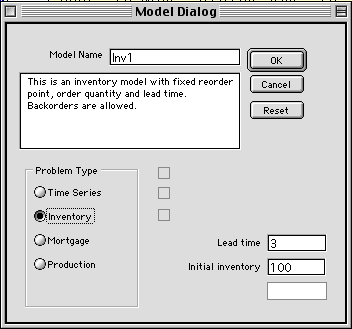
There are no options available with this model except
the lead time and Initial inventory. They are specified
on the dialog. The initial inventory may changed on the
worksheet, but the lead time affects the simulation structure.
Once defined here it cannot be easily changed.
|
|
The Worksheet Model
 |
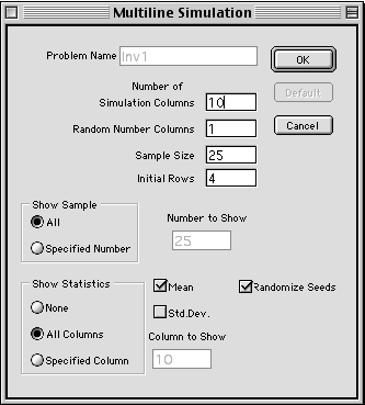
Pressing the OK button on the model dialog, brings forth a
second dialog that provides the features of the multiline simulation
model that will describe the process. The problem name is fixed
as the name given in the Model dialog and the parameters are
set to their proper values. The numbers of columns may be increased
to accommodate additional model features, but they should not
be reduced or the program will not be able to build the inventory
model.
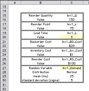
Pressing OK for this dialog, builds the worksheet
for the inventory model. All expressions are automatically placed
in row 1 and the random variable and parameter definitions are
placed on the worksheet. The figure below shows the parameters
that affect the inventory model and the definition of the random
variable for demand. A simple time series model is used in this
case without trend or step components. The parameter and random
variable definitions are placed in columns B and C. Note that
the lead time parameter is shown in yellow. This indicates that
the lead time should not be changed. Actually, changing the
lead time here will not affect the results because it is fixed
in the expressions defining the system.
|
| |
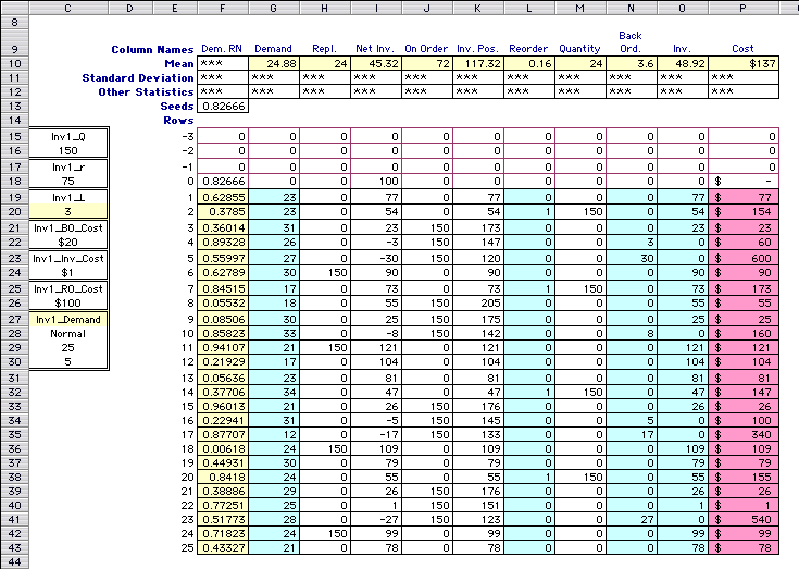
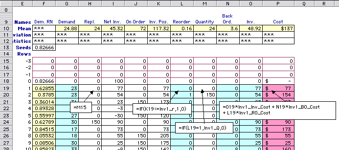
The simulation model is shown below. This model has a single
random variable for demand, shown in column, F. The columns
necessary for the simulation are columns G through P. The model
is complete and the simulation for 25 days is shown in the figure.
The interesting result is in column P that shows the average
cost per day. The other columns are necessary to determine the
replenishment orders, backorder amounts and inventory amounts.
|
|
Row 1 for the Simulation
|
| |
Row 1 for the simulation is row 19 on the worksheet. We identify
several interesting cells on this row.
|
| |
|
Cell
|
Description |
|
I18
|
This cell holds the initial inventory
amount. It may be changed, as well as the other cells in
the initial rows of the model. |
|
H19
|
This cell is interesting because it points several rows
higher (earlier) in the simulation. Cell H19 represents
the replenishment amount received in day 1 and points
to the order quantity that occurred four days earlier
(in cell M15). We are assuming here that orders are placed
at the end of the day and are available for sale three
whole days later. The amount will be available for sale
during the fourth day following the order.
In general, expressions may point to any cell that describes
the system earlier in time. It is necessary to provide
one more initial row than the lead time. Otherwise the
expression would point to a non-numerical cell.
Expressions may also point to cells in row 1. It is good
practice to only point to cells to the left in row 1.
Otherwise it is possible to create circular references.
This is not allowed by Excel. It is not reasonable to
point to cells lower (later) in the simulation. Circular
references will almost certainly be created.
|
|
L19
|
This cell holds an "IF" expression, that returns
1 if the inventory position in cell K19 is less than the
reorder point. Thus it indicates if an order will be placed.
|
|
M19
|
This cell holds an expression that places the order quantity
into the cell if the previous cell L19 is 1.
|
|
P19
|
This cell computes the cost per day based on the cost
parameters and the decision to order, the backorder amount
and the inventory amount. Both of the latter are computed
at the end of the day.
|
By increasing the sample size, the model can be simulated for
a large number of days to determine the average cost of operating
the inventory.
At the top of the worksheet, the add-in has added summary information
about the simulation run. The summary is gathered from important
information from the statistics rows.
|

|


