Consider a directed graph consisting of n nodes. There is an arc between every pair of nodes, so the graph is said to be complete. A directed spanning tree consists of n-1 arcs selected so that the arcs define a unique directed path from a designated root node to every other node. The figure below shows a tree with 7 nodes where node 1 is the root node. The Tree combinatorial problem Tree-COP deals with problems that must choose a directed spanning tree. The model can be specialized to three cases that have a long history in applied optimization and OR: spanning tree, path tree and flow tree. The Optimize add-in deals with the general forms for these problems. The Combinatorics add-in provides less general but more efficient treatments for the spanning tree and path tree problems.

The general Tree-COP seeks the tree that maximizes or minimizes an arbitrary objective function, perhaps limited by constraints.

It is clear that an arbitrary vector of integers for x will not necessary form a tree, so the number of trees is much fewer than the number of solutions for the general COP. For moderate n however, the number of directed spanning trees is still very large. It is fortunate that some well known specializations have polynomial solution algorithms.

We consider three special cases that differ according to the objective function: the spanning tree, path tree and flow tree. In each case below all trees are feasible, but the set can easily be restricted by adding additional conditions through the definition of G. The three versions of the Tree-COP are implemented in the Optimize add-in. All can be solved with either complete enumeration or heuristics. It happens that the greedy heuristic leads to the optimum solution of the spanning tree and path tree problems under certain conditions.

Spanning Tree

The spanning tree problem is to select arcs that construct a directed spanning tree so that the sum of the lengths of the selected arcs is minimized over all possible trees.

The Excel model for the spanning tree-COP with seven nodes is shown below. This model was constructed by the Combinatorics add-in with the length of an arc connecting two nodes computed with an Euclidean measure truncated to an integer value. The spanning tree problem with symmetric arc lengths can be solved to optimality with a greedy algorithm. For this case the greedy approach is equivalent to Prim's Algorithm. The highlighted cells show the arcs in the optimum tree. The solution vector is in range D9:J9.

The figure was constructed by the add-in to show the optimum tree rooted at node 1.

The figure below shows the minimal spanning tree that connects the 48 state capitals in the continental United States. Since distances are symmetric, the solution is optimum and the same solution is optimum for any root node. Since the greedy approach yields the optimum, this and larger problems are well within the capabilities of Excel.

For problems with asymmetric arc lengths or when G restricts the feasible solution, the greedy approach does not guarantee the optimum, so the problem is no longer in the set P.

Path Tree

The path tree problem is to select arcs so that the length of the path from node 1 to every other node in the tree is minimized.

The data structures of the spanning tree and path tree problems are different, but the algorithm used to find the solutions are the same. In both cases illustrated, the problems were solved to optimality by the greedy method. The difference between the two problems is that the greedy method was applied to different objective functions. The greedy method as implemented by the Optimize and Combinatorial add-ins is not the most efficient way to solve these problems. Many research papers have been published with faster implementations, but they are all polynomial.

We must note that the greedy method does not solve the path-COP if some arc lengths are negative. It happens however, that the 2-change improvement method will reach the optimum from an arbitrary starting tree.

Flow Tree

The flow tree problem is to select arcs so that the cost of the flows on the arcs is minimized. Flow is withdrawn from the nodes in specified amounts. The flow is supplied at node 1 and passed through the arcs of the tree.

Both the spanning tree and path tree problems are special cases of the flow tree problem. This form accommodates problems where the cost of flow is a nonlinear function of the amount of flow. When the cost is linear with flow, the problem is a linear path problem. Frequently, the problem of constructing a least cost flow distribution network will have concave costs. For this case, the optimum considering all flow paths is a tree. For problems with convex cost functions, the optimum solution of the flow problem is not generally a tree, although the Flow Tree-COP attempts to find the optimum when the solution is restricted to a directed tree.

In this model, the flow on an arc is the flow leaving the terminal node of the arc, j, plus the flow on all tree arcs leaving node j. This model is not as familiar as the spanning tree or path tree models, but it is a useful generalization in many instances.

An example is shown below with symmetric random data. One additional parameter is required for this model and is placed in cell F4. This is an exponent (Exp.) that will be used in the objective function. For a minimization problem the exponent will be between 0 and 1, inclusive.

The form constructed by the Optimize add-in for this problem is shown below. Several new rows appear in the form for a flow tree. The coefficients for the arcs are placed in the table starting in row 14. Row 8 holds the node flows and row 9 holds the arc flows. The node flows are data items which for simplicity we make all 1's for the example. In general the node flows should be nonnegative numbers. The value of p is in F4, and it is 0.5. This is equivalent to multiplying the coefficient by the square root of the flow.

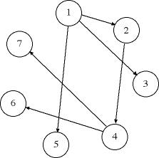
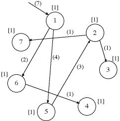
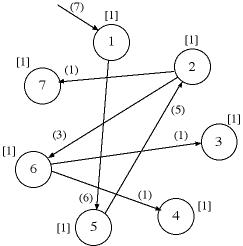
To explain the problem we use the solution shown in row 7. Recall that the value of a variable tells the node that originates the arc that enters a particular node. For example x2=5 implies that arc (5, 2) is part of the tree. The initial tree is illustrated in the figure below. The node flows are shown in square brackets on the figure and the arc flows are in parentheses. The node flows may be viewed as demands for some material at the nodes. The tree arcs are to deliver the demanded quantities and the materials enter the network at the root node (node 1). The flow in the tree arcs are determined by conservation of flow. For example, since the arc (2, 3) serves only node 3, the flow on this arc is 1. Arc (5, 2) serves nodes 2, 3 and 7, so it must carry 3 units of flow.

Given the tree designation in row 7 on the worksheet, the arc flows are computed in row 9 by Excel formulas. Row 10 holds the unit costs for the arcs selected for the tree. Row 11 computes the product of the unit cost multiplied by the arc flow raised to the power of the exponent. The sum of the values in row 11 is in cell D3 and is the objective to be minimized.

When the exponent is strictly between 0 and 1 and the coefficients are positive, the objective is a concave function of flow. This kind of problem is difficult because the associated math programming model has multiple local minima. For the math programming model, every tree is a basic solution and every basic solution may be a local minimum. Thus the flow problem for exponents strictly between 0 and 1 is hard and must be solved by combinatorial methods.

We use exhaustive enumeration for the example problem and the optimum solution is shown below.

The optimal tree is shown in the graphic.