We consider now a tree problem that is not as simple as the minimal spanning tree or shortest path tree problems in that greedy or improvement algorithms cannot guarantee optimum solutions even when the arc costs are nonnegative. For this tree problem, the tree arcs carry flow and the objective function is a concave function of arc flow. This is called the Flow Tree problem. We will see that the minimal spanning tree and shortest path tree problems are special cases of the flow tree problem. To illustrate the problem we construct a combinatorial form for a network with 7 nodes.

An example is shown below with symmetric random data. One additional parameter is required for this model and is placed in cell F4. This is an exponent (Exp.) that will be used in the objective function. For a minimization problem the exponent will be between 0 and 1, inclusive.

Several new rows appear in the form for a flow tree, row 8 holds the node flows and row 9 holds the arc flows. The node flows are data items which for simplicity we make all 1's for the example. In general the node flows should be nonnegative numbers.

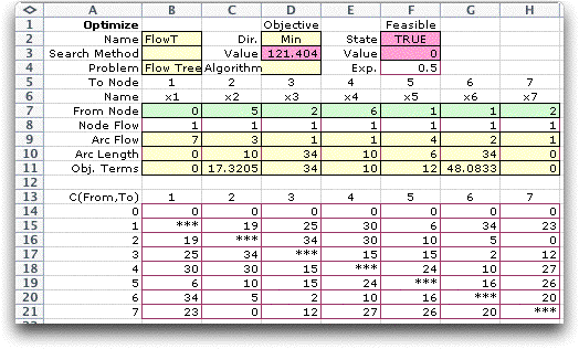
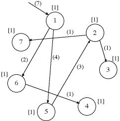
To explain the problem we use the solution shown in row 7. Recall that the value of a variable tells the node that originates the arc that enters a particular node. For example x2=5 implies that arc (5, 2) is part of the tree. The initial tree is illustrated in the figure below. The node flows are shown in square brackets on the figure and the arc flows are in parentheses. The node flows may be viewed as demands for some material at the nodes. The tree arcs are to deliver the demanded quantities and the materials enter the network at the root node (node 1). The flow in the tree arcs are determined by conservation of flow. For example, since the arc (2, 3) serves only node 3, the flow on this arc is 1. Arc (5, 2) serves nodes 2, 3 and 7, so it must carry 3 units of flow.

Given the tree designation in row 7 on the worksheet, the arc flows are computed in row 9 by Excel formulas. Row 10 holds the unit costs for the arcs selected for the tree. Row 11 computes the product of the unit cost multiplied by the arc flow raised to the power of the exponent. Rows 9 through 11 are colored yellow to remind the user not to change these cells.

The objective function for this problem raises the flow to the power of the exponent given in cell F4 and multiplies the result by the coefficient in the objective coefficient table. Since the example uses the exponent 0.5, this is equivalent to multiplying the coefficient by the square root of the flow. This value is computed for each arc in row 11. The sum of the values in row 11 is in cell D3 and is the objective to be minimized.

The minimal spanning tree problem and the shortest path problem are special cases of the flow tree problem. With the exponent at 0, an arc with nonzero flow contributes exactly the arc coefficient to the objective since any positive flow raised to the 0 power is 1. Thus, solving the problem with a 0 exponent will obtain the minimal spanning tree. With the exponent 1, an arc with nonzero flow adds to the objective the arc coefficient multiplied by the flow. This is the same contribution that an arc adds to the objective for the shortest path tree. Thus, solving the problem with the exponent 1 obtains the shortest path tree. We illustrate these two solutions later.

When the exponent is strictly between 0 and 1, the objective is a concave function of flow, assuming positive coefficients. This kind of problem is difficult because the associated math programming model has multiple local minima. For the math programming model, every tree is a basic solution and every basic solution may be a local minimum. Thus the flow problem for exponents strictly between 0 and 1 is difficult and must be solved by combinatorial methods.

We use exhaustive enumeration for the example problem with the best 20 solutions shown in the table below.

The optimum solution is pictured below.

The combinatorial form shows the optimum.

Greedy Solution and Heuristics

We use the same greedy approach used for the other tree problems. The solution is constructed by starting from the root node and adding the arc that makes the smallest contribution to the objective. The first arc carries 1 unit of flow, so the arc leaving node 1 with the smallest coefficient is added to the tree. This is arc (1, 5) so the tree now has nodes 1 and 5 and arc (1, 5). The second step adds an arc that leaves either node 1 or node 5 and does not make a cycle. The arc to add is the one that increases the objective the least. The result of this step is not so obvious since an arc leaving node 1 adds the its coefficient directly, but an arc leaving node 5 adds the coefficient but also the affect of changing the flow on arc (1, 5) from 1 to 2. The greedy approach adds arc (5, 2) at the second step. The process continues adding one node and one arc to the tree at each step. The criterion is to minimize the objective at each step. Since this is a greedy algorithm, the process stops when all nodes are in the tree. The results of the greedy algorithm are shown below. In this case the optimum was obtained, but this result is not guaranteed.

We illustrate the improvement process by starting from the solution given at the top of this page. The results are below. The initial solution is at the bottom of the list and subsequent improved solutions appear above it. The improvement approach is the same as for the other tree problems. Each nontree arc is inserted in the tree and the current solution arc terminating at the same node as the entering arc is deleted. If a cycle is not formed, the solution is evaluated. An improved solution replaces the current incumbent. Again the optimum solution is obtained for the example, but there is no guarantee of this result.

In general the flow tree problem is not surely solved by either the greedy approach or the improvement approach. The optimum can be obtained by exhaustive enumeration, but that is impractical except for very small problems. One can write an integer programming model using piecewise linear approximations for the convex objective function terms, but again cycles are a problem and the model is not simple. The analyst faced with this problem must be satisfied with a heuristic solution perhaps obtained with a combination of random searches and improvement steps.

The flow tree problem may have node flows other than 1 and may have a more complex objective function. A practical problem might seek an optimum pipe layout for collecting oil from well sites located in a geographic area. The cost of an arc would be the cost of the pipe necessary to carry the flow served by the arc and this might be a complex function involving discrete pipe sizes. One would expect economies of scale with regard to pipe cost versus flow. The combinatorial methods of solution are not limited by such added model complexity since the methods do not depend on simplifying assumptions.

Relation to Shortest Path and Minimal Spanning Tree

The flow tree problem is interesting because it is a hard problem bracketed by two easy problems. For symmetric-nonegative coefficients the problem with the exponent equal to 0 can be solved to optimality by Prim's greedy algorithm, while the problem with the exponent equal to 1 can be solved to optimality by Dijkstra's greedy algorithm. The two results are obtained with the add-in for the same data below. First we set the exponent to 0.

It happens that he minimal spanning tree obtained is the same as the optimum with the exponent equal to 0.5.

Setting the exponent equal to 1 and solving with the greedy algorithm we find the flow solution below.

The shortest path tree obtained is different than the solution with the exponent equal to 0.5.