|
|
 |
Building
a Simulation |
 |
To
build a simulation, choose the Build Sim item from the
Simulation menu. |
 |
|
|
For this introduction we are simulating
a simple time series that represents the demand for some
product. The model for the time series is described mathematically
in the figure below.
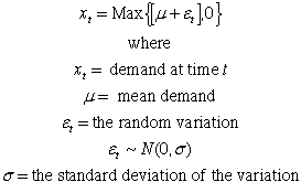
The demand is based on a specified mean
demand and the standard deviation of the random variation
term. The variation is Normally distributed with a mean
value of zero. We require that the time series return
a nonnegative integer as indicated by the brackets in
the top expression.
|
|
| |
| The Build Sim option calls
a VBA program that presents the dialog shown below. The
dialog requires a name. We provide the name TS1. The name
should be short and representative of the model. The name
must start with a letter, have no spaces and include no
punctuation except the underline symbol (_). The four fields
under the name determine the number of rows and columns
of the display. |
|
Building the Simulation Form
 |
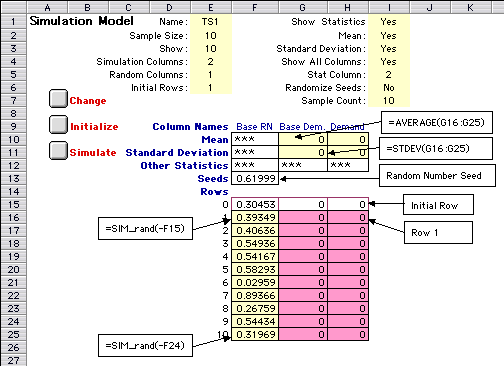
The worksheet constructed by the add-in is shown below. The
sheet has the name TS1. Since several ranges on the sheet are
given names prefaced by the worksheet name, the name can not
be changed once the sheet is constructed.
Notice that the display has three columns, the first is labeled
"Base RN", and the other two have the labels "Base
Dem." and "Demand". These are the Random Number
columns and Simulation columns, respectively. Their
number of columns of each type are determined by the associated
fields on the dialog. The columns originally had default names
that were changed to represent the current problem.
At the very top of the display, we see parameters obtained
from the dialog box. They are colored yellow to indicate that
they should not be changed by the user. The rows beginning at
row 9 and continuing through row 13 hold statistics for the
simulation. Row 15 is the initial row and holds numbers that
initialize the formulas of the simulation. Only one initial
row is shown, but the number is controlled by the Initial
Rows field of the dialog. Row 16 of the worksheet holds
row 1 of the simulation. This is an especially important row
as it contains the formulas that describe the situation being
modeled. The nine rows starting with row 17 are the remaining
iterations of the simulation. The Sample Size field of
the dialog determines how many rows are in this category.
Most of the structural features of the display are modified
by clicking the Change button located in column A. Then
the dialog above is again presented. All the fields on the dialog,
except the name, can be changed by specifying new values on
the dialog.
|
 |
The contents of several cells are expanded with the outlined
text boxes in the figure above.
|
Cell
|
Description |
|
F10
|
This cell is in a random number
column of the statistics display. Its content,"***",
indicates that statistics concerning this column are not
maintained. Generally, the add-in does not maintain statistics
about random number columns. |
|
G10
|
This cell holds the Excel function.:
=AVERAGE(G16:G25)
It computes the average, or the statistical
mean, of the simulated numbers in the Base Dem. column.
Cell H10 holds a similar function for the Demand column.
The contents of the cells in this area are controlled
by the Show Statistics area near the bottom left
of the dialog. Buttons are provided that determine if
statistics are shown at all, if the mean is to be shown,
if the standard deviation is to be shown, if all simulation
columns are to be computed or if only one. When a single
column is to be specifed, there is a field on the dialog
in which the column index is to be specified. Note that
the number used in this field is the simulation column
number.
|
|
G11
|
This cell holds the Excel function that computes the
standard deviation of the simulated numbers in the Base
Dem. column:
=STDEV(G16:G25)
A similar function is provided in cell H11
for the Demand column.
|
|
G12
|
This cell is provided for the user to specify some other
statistical function than "AVERAGE" or "STDEV".
There are a number of statistics one might like to gather
and Excel has a variety of functions for this purpose.
|
|
F13
|
This is a "seed" for
the random numbers in the column below F13. The seed is
initially obtained using a random number generated by Excel,
but the seed may be changed by the user. For a positive
seed, the sequence of random numbers will always be the
same. This is useful for some applications. If the Randomize
Seeds button is checked on the dialog, the program randomly
generates a new seed for every run of the simulation. |
|
F15
|
When a simulation is run, the
seed in F13 is transferred into cell F15. This in turn controls
the sequence of random numbers below F15. |
|
F16
|
Here we see a User-Defined function:
=SIM_rand(-F15)
The function is provided by the Simulation
add-in and has the purpose of generating a uniformly distributed
random number between 0 and 1. The function uses the random
number generator provided by Excel. Notice that the function
points to cell F15. This provides the connection between
the random number generated and the seed. The function
requires a negative argument, thus we negate the reference
to F15.
|
|
F25
|
This cell is in the last row of the column and holds
the function:
=SIM_rand(-F24)
Thus the contents of cell F25 depend on the contents
of cell F24. All the cells from F16 through F25 have the
same relative reference, so all are controlled by the
seed at the top of the column.
|
|
F15:H15
|
This range is the initial row, which
is labeled row 0 in this case. The random columns will
hold the seeds in this range. The simulation columns will
hold initial values for the simulation. For example, an
inventory model would require an "initial inventory"
quantity. This would be placed in an appropriate column
in the initial row. Some models will require more than
one initial row.
|
|
F16:H16
|
This important row holds the
formulas that describe the simulation model. The random
columns are filled by the computer, but the simulation columns
must be filled by the user. For some systems, the formulas
in these cells may be very complicated. The complexity of
the situation that can be modeled depends a great deal on
the inventiveness of the user and the user's skill at manipulating
Excel formulas. |
|
| Filling Row 1 |
| |
The simulation columns of row 1 hold formulas that define the
iterative simulation model. The model can be very complex since
Excel allows about 250 columns of formulas. For example a multiline
simulation model of a three channel queue constructed by the
Queueing add-in has 19
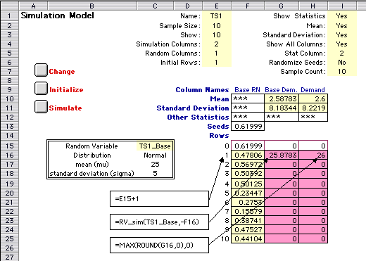
columns. Below we show the contents of row 1 for the example
time series model.
|
 |
The model for the time series example is placed in two cells
in row 1, cells G16 and H16, Cell E16 holds the row index, which
is also computed with a formula.
|
Cell
|
Description |
|
E16
|
This cell holds the row index. The cell holds the simple
expression
=E15+1
The index is one greater than the contents
of the row above. Since the index of the initial row is
0, the index of this first row is 1. This formula is automatically
provided by the add-in, but it can be changed by the user.
For example if the simulation was to show 10 day intervals,
the formula could be
=E15+10.
|
|
G16
|
This cell computes the value of

Notice that in range (B15:C18) we have defined
the random variable "TS1_Base". The cells in
this range were filled by the Add RV command of
the Random Variables add-in. The distribution is
specified as a Normal distribution with mean 25 and standard
deviation 5. Simulating from this distribution is accomplished
in cell G16 with the function:
=RV_sim(TS1_Base,-F16)
RV_sim is a user-defined function
provided by the Random Variables add-in. That add-in must
be installed in order for this function to be available.
The example illustrates the arguments of the function.
The first argument is the random variable name and the
second is a seed. The seed for the cell G16 points to
F16, the cell just to the left. The argument is negated
so that the value of the random variable is determined
by the seed.
If the mean or standard deviation stored
in cells C17 and C18 are changed, the number in cell G16
changes accordingly. The Random Variables add-in provides
a large variety of discrete and continuous probability
distributions.
|
|
G17
|
This cell completes the computation of the required time
series value for t=1.

The Excel expression in cell G17 is
=MAX(ROUND(G16,0),0)
where the ROUND function converts the contents
of G16 to an integer and the MAX functions assures that
it is nonnegative.
The contents of cells G16 and G17 could
have been combined into a single column for this simple
example.
|
|
|
Performing the Simulation
|
| |
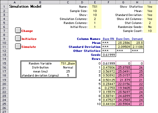
Clicking the Simulate
button copies the formulas in row 1 into rows 2 through 10. Since
relative addresses are preserved, each row computes the values
for one iteration. The simulation statistics are computed in rows
10 and 11 for the sample. |
 |
When developing a model, it is good practice to keep the sample
size small. Here we have used 10 iterations. During the development,
the user often will add and delete columns. This is easily accomplished
with the Change button. When columns are inserted they
are added in a manner that does not invalidate functions or
references already created.
When the model is perfected however, a larger sample size is
necessary to obtain statistically valid results. Again, this
is easily accomplished by changing the sample size in the dialog
(reached with the Change button). The add-in automatically extends
the model by inserting rows and filling the rows with the expressions
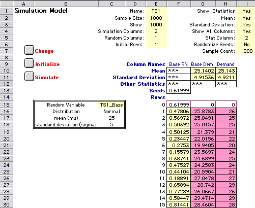
in row 1. The figure below shows the results for 1000 iterations.
Since Excel allows very many rows in the model, the sample size
can be very large. We later describe a procedure that uses a
large sample size, but displays only a relatively small number
of iterations.
|
 |
A simulation model created
by this procedure is dynamic. Cells are linked to each other by
active formulas. When a random number seed or a problem parameter
is changed, the entire simulation responds. This allows a variety
of analysis procedures not usually available with a simulation
model. We review these possibilities more fully on a later page. |
|


