|
|
 |
Portfolio |
 |
-Capital
Budgeting with Risk
|
 |
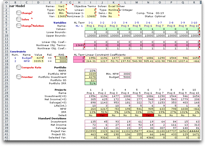
The capital budgeting
model considers risk by computing the statistical variance (and
standard deviation) of each project and either minimizing the
portfolio variance or placing a constraint on portfolio variance.
When risk is considered, the initial investment, net income,
and salvage value of each project are assumed to be random variables
with specified mean values and standard deviations. For this
analysis the life of a project is not a random variable, but
is a fixed value. Although it is sometimes convenient to assume
Normal distributions for the random variables, it is
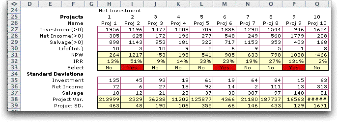
not necessary for these results. The data for the projects in
an example problem are shown in the table below. For the example
we assume that all random variables are statistically independent.
The mean values for the investment, net income and salvage
are given for the example in rows 27 through 29 and the corresponding
standard deviations are given in rows 35 through 37. The project
lives are in row 30. |
|
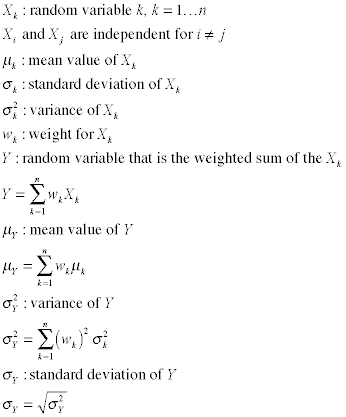
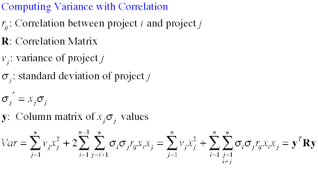
It is easily shown
using basic definitions that the weighted sum of independent
random variables is a random variable whose mean and variance
can be calculated as below.
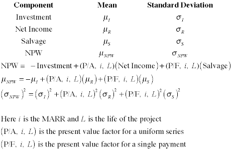
Since the present worth values are computed as
a weighted sum of the components, the mean and variance for
the NPW for each project are computed as below.
Row 31 in the table above holds the values of
the mean NPW for each project and row 38 holds the values of
the variance for each project. The variance for Project 10 is
too great to display with the current column width. Row 39 is
the square root of row 38, and holds the standard deviations
of the projects.
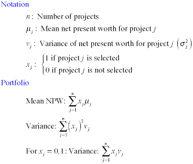
Using the same principles, the mean and variance
of the portfolio can be expressed as functions of the decision
variables.
The portfolio variance is a nonlinear function
of the decision variables, but when the values or the decision
variables are restricted to 0 and 1, the variance can be expressed
as a linear function. We use the linear expression in models
with the 0-1 restriction. This allows models to be solved using
linear-integer programming rather than nonlinear-integer programming.
The latter is much less reliable than the former. |
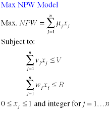
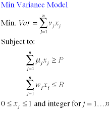
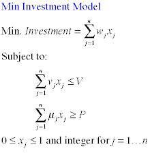
Math Programming Model |
|
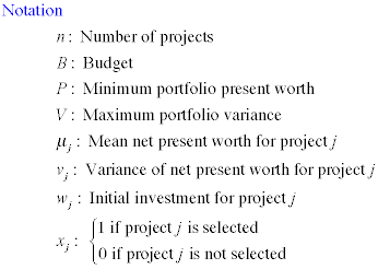
With these definitions, several
optimization models are possible depending on the goal of the
analyst and the constraints that are included. We can maximize
the NPW while placing an upper bound constraint on the variance,
we can minimize the variance while placing a lower bound constraint
on the NPW, or we can minimize the initial investment while
placing constraints on both the variance and the NPW. In each
case we assume that the model includes a budget constraint.
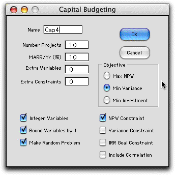
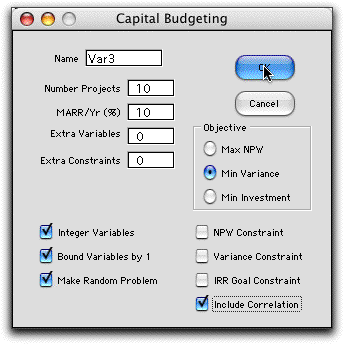
The options are set on the Capital Budgeting dialog.
The figure below shows the three models when the
selection variables are limited to 0 or 1, representing not
select or select. Since all the models are linear,
integer-linear programming can be used to find the optimum portfolio
of projects. |
| |
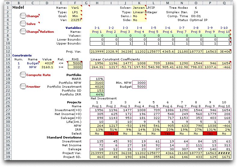
The worksheet below
shows the minimum variance solution for the example. Cells K21
and K22 are provided to hold the minimum NPW and the Budget
respectively. These are controlled by the analyst. Of course
when the cells are changed the model must be solved to obtain
the new solution. |
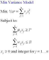
Nonlinear Model
|
|
When variables are
allowed to assume values greater than 1 or the integrality restriction
is dropped, the optimization model is nonlinear.
The add-in creates the nonlinear-integer model below when the
variables are not restricted to binary values. Cell H13 holds
a nonlinear term than is the sum of the variance multiplied
by the values of the squared number of projects. The optimum
selects two of project 2 and one of project 6. Since the variable
values are squared, the solution tends to have solutions with
several selected projects rather than several copies of the
same project. In the example two units of project 2 are selected
because it has such a low variance. The model is both nonlinear
and integer. The Excel Solver can solve such models, but the
performance is much reduced in comparison to a linear-integer
model. If the Solver fails to find a feasible solution, it is
always a good idea to try alternative initial solutions. We
have used the variable values 1/n with some success. |
Efficient Frontier
|
|
By sequentially solving
this problem with different limits on the NPW constraint, the
analyst can construct a set of solutions each with the minimum
variance for the obtained value of the NPW. We illustrate with
the model having binary variables. We set the budget for the
example problem to be very large and not constraining and solve
the problem for increasing limits on the NPW. A set of solutions
is obtained. Plotting the solutions on a chart with NPW and
variance as the axes, one obtains what is called the efficient
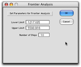
frontier of solutions. To find the efficient frontier click
the Frontier button on the worksheet. The program finds
the lower limit by setting the NPW constraint limit to 0 and
solving the model. The lower limit obtained is the NPW of the
minimum variance portfolio. The upper limit is the sum of the
positive project NPW values. To make a more refined search,
these limits may be changed. The Number of Steps entry
specifies how many individual problems are solved. The NPW range
is divided into this number of equal intervals.
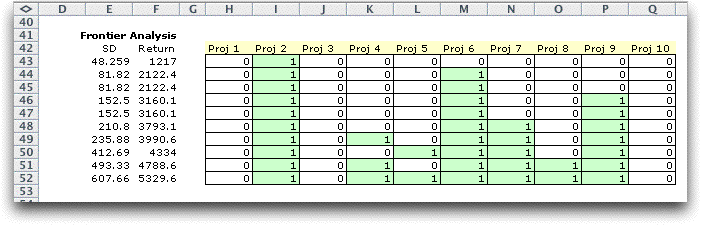
The model being solved is a linear-integer programming
model. It is solved 11 times. Excluding the last value for which
the program cannot find a feasible solution, we obtain the solutions
in the table below. Green cells indicate nonzero values.
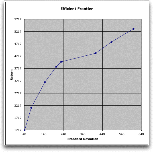
A graph of the efficient frontier appears immediately
below the table. We connect the individual points with straight
lines, but since a finite number of solutions are generated
this is only an approximatin of the frontier. If the entire
frontier were available, any solution not on the efficient frontier
is dominated by some solution on the frontier. There are portfolios
with values that appear below the frontier, but none that are
above. With continuous decision variables the frontier has a
concave shape. With discrete variables, the shape may not be
concave. Since the NPW values are chosen with fixed size steps,
the curve may not show all solutions on the frontier. Also different
values of NPW may yield the same solution.
The same solutions will be found by maximizing
the NPW with a constraint on the maximum variance, however the
automatic feature of the program is only available when minimizing
the variance. |
Correlation
|
|
It is conceivable that projects
are not statistically independent. The returns of dependent
projects are related through a correlation matrix. To form a
model with correlation, click the appropriate checkbox in the
dialog.
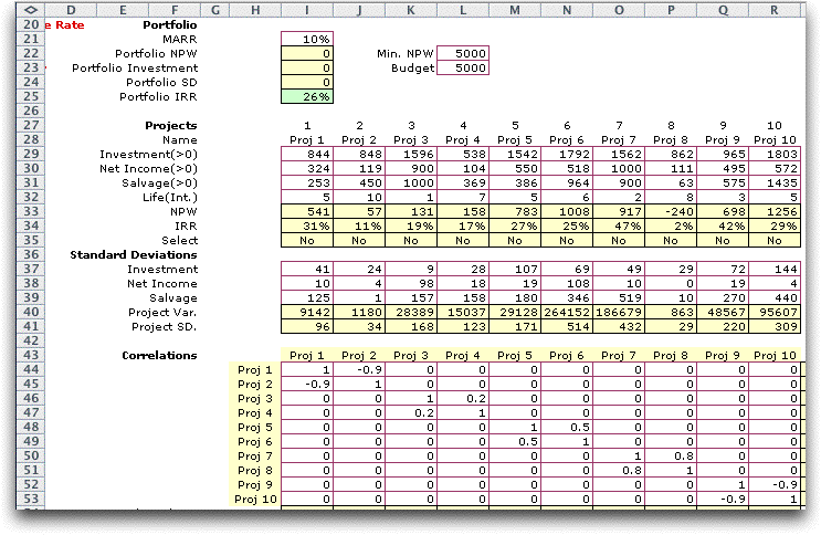
The data for a correlated model is shown below.
A correlation matrix is included below the return and variability
data. A valid matrix has 1's on the diagonal, is symmetric and
has numbers between -1 and +1 on the off-diagonals. The resultant
matrix must be positive definite.
This matrix is filled by the modeler with information
concerning the correlation between projects. We have illustrated
the situation by providing nonzero correlation coefficients
between pairs of projects. Note that we have included a large
negative correlation coefficient between the pairs (1, 2) and
(9, 10). For selected projects with negative correlation, the
statistical variability tends to cancel out. |
|
|
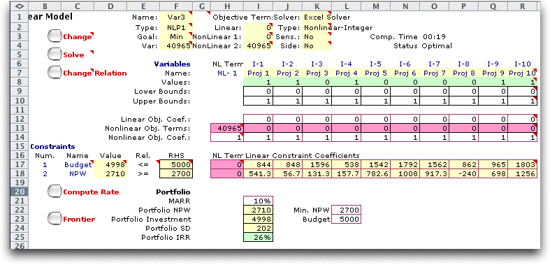
The variance of the
portfolio is a nonlinear function of the decision variables
as shown below. The portfolio variance function is used in the
several model formulations when correlation is part of the model.
A related result is used extensively for Markowitz
portfolios considered on the next page.
The solution for the example is shown below. Note that the
two pairs of negatively correlated variables are both used in
the solution. Actually the solution shown was obtained with
some difficulty. The Solver often does not find exact solutions
for nonlinear-integer programming problems. |

|