|
|
 |
Combinatorics |
 |
-Sequencing
Problem |
| Shortest Processing
Rule Example |
| |
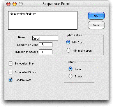
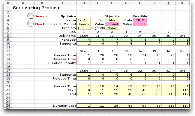
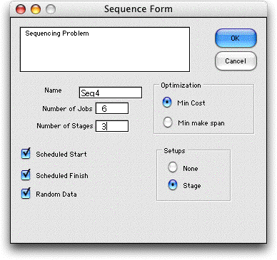
To model a sequencing problem, choose Sequence
from the Combinatorics menu. We start with a simple
case described by the dialog below. The problem has 6 jobs that
must pass through a single stage of production. No setup time
is required and there are no early or late schedules. These
variations are illustrated later.
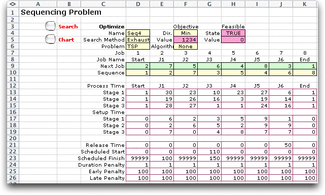
The worksheet is constructed using random data for job processing
times. Two extra jobs are included. A start job is
indexed 1 and an end job is indexed 8. The six jobs
required by the dialog are indexed 2 through 7. The solution
to this problem is a sequence beginning at start and
passing through the six jobs and terminating at end.
The variables defining this sequence are the next jobs
listed in row 9 of the worksheet. The initial sequence performs
the jobs in numeric order.
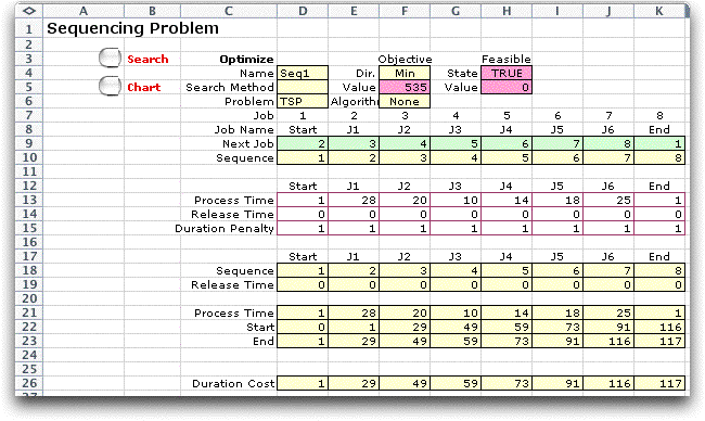
The solution to this problem is a tour so the form
below identifies the problem type in cell D6 as a TSP. This
cell is used by the Optimize add-in to control the
search process. The other cells in rows 4 through 6 are used
by the add-in and generally should not be changed. Cell F5 holds
the formula for the objective function. Although the proper
formula is provided for the problem at hand, the modeler may
change the formula to represent features not modeled. Cells
H4 and H5 hold feasibility conditions. The formulas provided
require that all the entries in row 9 be greater than 0. Other
feasibility conditions may be added by the modeler. |
| |
The data items for this example are the process
times, the release times and the duration penalties, entered
in rows 13, 14 and 15 respectively. A job occupies the production
stage for the process time. The release time is the time that
a job is available to begin processing. The duration penalty
is multiplied by the job completion time to determine the objective
value for a solution.
Computed quantities are presented in rows 17 through 26. Rows
17 through 19 and row 21 sort the data according to the current
sequence. When the sequence corresponds to the job indices,
as shown, the data is simply repeated on these lines.
Rows 22 and 23 computes with Excel formulas the start
time and end time of each job for the given sequence.
Row 26 computes the cost for each job by multiplying the completion
time by the duration penalty. For this simple case, all duration
penalties are 1, so all jobs are equally important with respect
to completion time.
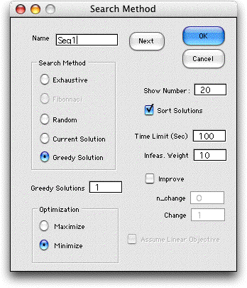
The subroutines of the Optimize add-in are used to
find solutions to this combinatorial problem. When all the jobs
have the same duration cost, a greedy solution found by selecting
the shortest job first is the optimum. This is the default greedy
algorithm for the Optimize add-in. To call the appropriate
dialog, click the Search button on the worksheet. The
dialog below is presented. |
| |
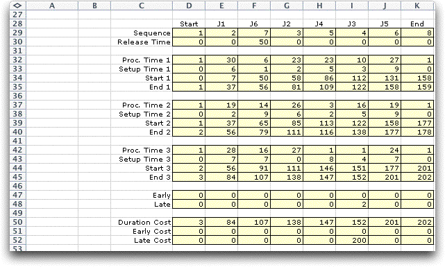
The results of the greedy process are shown
below. Now the rows starting at row 17 present the job information
sorted in order of the solution. The processing times on row
21 follow the SPT, the shortest processing time, rule.
This is optimum when all duration penalties are 1 and there
are no additional constraints on the solution. |
| |
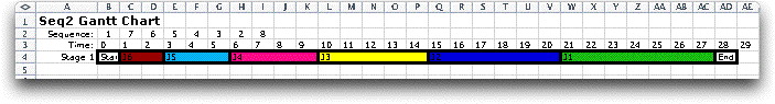
The Chart button creates
a Gantt chart of the solution. Either a vertical or horizontal
presentation is allowed. Since the worksheet has 256 columns
and over 65,000 rows, the vertical presentation is usually preferred.
A column or row is required for each time interval. The total
time for the example is too long to display on this page, but
we show below the Gantt chart for an smaller example. The chart
is created on a separate page from the data. The start and the
end cell are colored white. The job cells are colored based
on the index of the job. In order for a job to appear, it must
have a processing time of at least 1. We have specified the
processing times of the start and end as 1 so that they appear
on the chart.
|
Example with Stages
| |
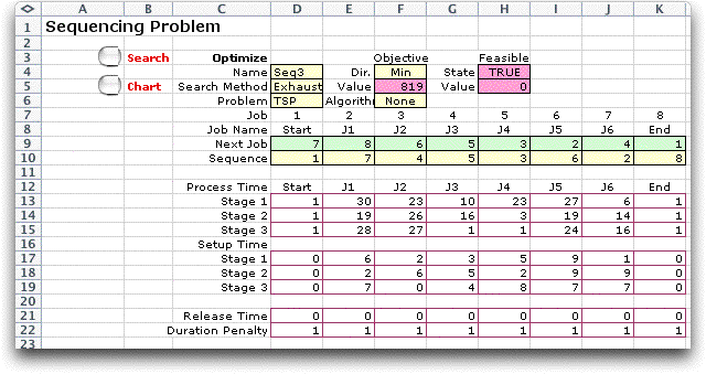
It may be that a job may be required to pass through several
stages of a production process. A system of this type is a flow
shop since we are assuming that every job passes through
all the stages, and the sequence of jobs at each stage is the
same. To illustrate stages and setup times we create
a second example.

The data for the example is shown below. The solution
is obtained with exhaustive enumeration, only possible because
the problem has only six jobs. |
|
| |
The computed results for
the optimum solution are below. The finish time for the
jobs are the end times for stage 3 of the system. There
are two restrictions on when a job may begin at some stage.
The job cannot begin on a stage until the setup and processing
times for all previous jobs on that stage are complete.
Also a job cannot begin on a stage until the job is finished
on the previous stage. At stage 1, a job cannot begin
until its release time. When both the restrictions are
satisfied, the job begins. |
| |
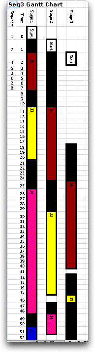
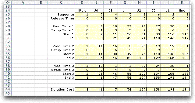
The effects of setup times
are illustrated by the partial Gantt chart at the left.
The first job (after start) is job 6 with a setup
time of 1 and a processing time of 6. Setup times are
in black and job 6 has the brown color in the Gantt chart.
Although stage 1 processing is complete and job 6 is available
for stage 2 at time 7, it cannot begin processing at stage
2 because of the setup time of 9 periods for job 6 at
stage 2. Note that we are assuming that a job can be setup
for the next stage during an idle time before the job
actually is available. After completion of stage 2, job
6 can immediately begin on stage 3. The setup time for
job 6 on stage 3 is performed before job 6 arrives. There
are some time intervals near the bottom of the figure
with no color. During these periods the stages are idle.
For example stage 3 is idle for one period from time 41
to 42. Job 3 does not arrive until time 46 and the 4 periods
of setup time need not begin until time 42. In general,
stage 1 will remain entirely occupied until all jobs are
complete in stage 1. Later stages may have idle times.
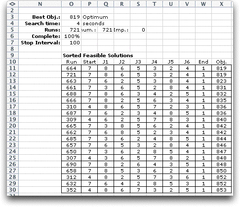
The exhaustive enumeration procedure generates and evaluates
all feasible solutions. The best 19 of these are shown
below. The optimum solution is evaluated twice.
|
Early Start and Late Finish
| |
We use the same data as
the last example, but allow scheduled start and finish
times by clicking the check boxes.
The data for the example is below. Rows
9 and 10 hold the optimum solution. The default value
for the scheduled start is 0 and the default value for
scheduled finish is a large number, so the default values
do not affect the solution. We have specified a scheduled
finish of 100 for job 1 and a schedule start and finish
for job 3 of 110 and 150. In addition we provide a nonzero
release time of 50 for job 6. All these restrictions are
violated for the optimum solution obtained in the last
section except the scheduled finish for job 3. |
| |
The results are shown in
the arrays starting at low 28. Row 28 has the optimum
sequence job titles and row 29 holds the associated indices.
The release times, process times and setup times are repeated
but sorted according to the solution. The start and end
times for the three stages are computed.
From the solution we see that job 6 begins processing
in stage 1 at time 50, exactly its specified release time.
Release times are hard restrictions in that a job cannot
be started on the first stage until it is released. Job
3 has a scheduled start time of 110. We see from the results
that the start time for job 2 is 112. The program penalizes
start times that are before the scheduled start but does
not penalize start times after the scheduled start. Row
47 shows a positive value if a job is started early, the
difference between the scheduled start and the actual
start in stage 1. Note that setup for the job may take
place before the job is actually started.
Finish times will be penalized if they occur after a
scheduled finish. For the example we see that job 3 is
finished (end for stage 3) at time 152. The scheduled
finish is 150, so the job is late by 2 periods. The lateness
is computed in row 48. The finish time for job 1 is 84,
well below the scheduled finish of 100, so this job is
not late.
Rows 50, 51 and 52 hold the costs computed for duration,
early start and late finish. The objective function value
is the sum of the yellow colored cells of these rows. |
| |
The combination of early
scheduled start and late scheduled finish is usually called
a time window for sequencing problems. This example treats
time windows as soft constraints. Early starts and late
finishes are penalized but not prohibited.
The results shown here were determined by exhaustive
enumeration. The same solution was obtained for 10 random
searches, each followed by the 2-change procedure. Some
combination of heuristic methods will be necessary for
larger problems. The number of columns on a worksheet
limit problems to about 120 jobs. Even heuristic methods
will have trouble with this size problem, because every
solution tested requires an evaluation of the worksheet. |
|
| |
| |

|
|