|
|
 |
Inventory
Analysis |
 |
Systems |
| |
|
Several WIP components combine
to form a system. Components are linked by the flow between
them and the add-in provides three general arrangements
by which they may be linked and two mechanisms by which
flow is engendered.
System models are defined by selecting the System
command from the Inventory menu. The top four
boxes on the system dialog hold the location, name, time
interval and the number of components in the model. We
use the rest of this page to describe the structure and
drive options. The models assume steady-state, deterministic
operation. Although some of the components use resources,
there is no scheduling of scarce resources. Although in
many ways the assumptions are not realistic, the models
should be useful in identifying the source and magnitude
of WIP accumulations and the resultant system cycle times. |
The structure and drive options are set with buttons on the
dialog. The structure determines the arrangement of the flow
paths in the system. For a line the flow passes through
the components in series. A tree either starts with
a single component and the flow diverges to multiple components,
or the flow starts with several components and converges to
a single output component. A network allows arbitrary
interconnections between components.
The drive option specifies the cause of flow through the process.
For the pull option, products are pulled from the outputs
of components. For the push option, items are pushed
into the inputs of the components.
The O/I Ratio button determines whether a component
will change the flow quantity as the flow passes from its input
to its output. In the examples linked to this page we will not
choose this option. For these examples, the flow that enters
a component will be the same as the flow that leaves. On the
Ratio page we illustrate cases where non-unity ratios
will be important to the models.
The seven different WIP components are shown in
figure below for a pull line. Since all components are placed
on the same data form, the row titles are not as explicit as
they are for only one component. The cells with x's indicate
the irrelevant parameters for some of the models. The setup
cost, setup time, processing time and maximum utilization are
not used for the delay, bank or lot size change components.
For every component the first variable row, row 12 for the example,
shows the input lot size and last variable row, row 14, shows
the output lot size. Between these two rows, row 13, the definition
of the variable depends on the type of component. For a delay
this cell holds the delay time. For the bank the cell holds
the bank amount. The cell is not used for the lot change component.
For all other components the cell is the processing lot size.
|
|
|
We discuss
each of the drive/structure options below. Click on the link
on the section title to go to a page showing Excel worksheets
with numerical examples. In the following we use operation
to refer to a WIP component.
|
|
The
line is a series of components that all carry the same flow.
The flow is either pushed from the first component or pulled
from the last. The two cases are illustrated in Fig. 1. Click
the link on the title at the left to see numerical examples.
For the line system, the difference between push and pull is
a philosophical difference since for given parameters, the results
are the same for either case. The distinction is important for
the tree and network structures. We provide the two cases for
the line structure for completeness. It is also easier to start
the discussion with the line structure because of its simplicity.
The term push is often used for systems driven by customers
who enter at the first operation to receive a series of services.
Push systems are sometimes analyzed by queuing analysis because
the interarrival time between sequential customers may be a
random variable. The service times are also usually random variables.
The term pull is used to describe manufacturing systems. A
product must pass through a series of activities that change
raw materials into finished items. The system is driven by the
demand for the product. Sales draw finished items from the last
operation. Although manufacturing often involves variability,
the schedule of activities is sometimes more controllable. The
Just-in-time scheduling philosophy implies that product is pulled
by demand, rather than pushed by raw materials entering the
system.
Since our models neglect scheduling and variability for the
most part, the distinction between push and pull is lost. Whatever
is pushed into the first operation will ultimately leave the
last, and whatever is pulled from the last operation must have
previously entered the first. |

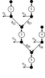
Figure 2
|
The generic pull tree is illustrated in Fig. 2. For this structure
the flow through each operation goes to a unique following operation,
while each operation may have several input flows from other
operations. This structure is appropriate for modeling manufacturing
processes where raw materials are combined or mixed to produce
a single product. Product is withdrawn or pulled from the operation
with the greatest index, operation 5 for the example, in an
amount specified in the data. In addition to the final operation
of the process, our models also allow flow to be pulled from
the other operations. These flows represent intermediate products.
In general, we identify the amount pulled from the output of
operation i as  ,
the pull flow at operation i.
For the tree structures we require that the operations be indexed
so that when flow passes from operation i to operation
j, i < j. The greatest index is
m. For the example m is 5.
For the pull tree we identify the proportion,  ,
as the amount of the output of operation i required
for each unit of product passing through operation j.
The value of
may be any positive amount to represent a variety of manufacturing
situations. An assembly operation that requires one unit of
each input to be combined to produce one unit of a subassembly
would have the proportions equal to 1 for each input. A mixing
operation that combines inputs into a mixture would have input
proportions that sum to 1. An operation that requires more than
one unit of some input would be modeled with a proportion greater
than 1 on the associated input. ,
as the amount of the output of operation i required
for each unit of product passing through operation j.
The value of
may be any positive amount to represent a variety of manufacturing
situations. An assembly operation that requires one unit of
each input to be combined to produce one unit of a subassembly
would have the proportions equal to 1 for each input. A mixing
operation that combines inputs into a mixture would have input
proportions that sum to 1. An operation that requires more than
one unit of some input would be modeled with a proportion greater
than 1 on the associated input. |
|
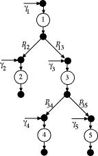
Figure 3 |
The generic push tree is illustrated in Fig. 3. For this structure
the flow into an operation comes from a unique preceding operation,
while the operation may have several output flows going to other
operations. This structure is appropriate for modeling service
systems where customers arrive at a source node, node 1 in the
example in the amount  .
In addition to node 1, flow may also be pushed into the network
at other operations. The flow entering at operation i
is .
In addition to node 1, flow may also be pushed into the network
at other operations. The flow entering at operation i
is  .
Note that push flow enters the process just before an operation. .
Note that push flow enters the process just before an operation.
The flow that passes through an operation may be split to go
to other operations to receive different types of processing.
Units pass through the tree until finally they are withdrawn
to the nodes that have no successors, nodes 2, 4 and 5 in the
figure.
For the tree structures we require that the operations be numbered
so that when flow passes from operation i to operation
j, i < j. The greatest index is
m. For the push tree we identify the proportion,  as the proportion of the output of operation i that
is passed to operation j. The value of
may be any nonnegative amount to represent a variety of situations.
For a splitting operation that separates the total flow passing
through operation i into several paths, the sum of
the proportions leaving i would equal 1.
as the proportion of the output of operation i that
is passed to operation j. The value of
may be any nonnegative amount to represent a variety of situations.
For a splitting operation that separates the total flow passing
through operation i into several paths, the sum of
the proportions leaving i would equal 1. |
| Pull
Network
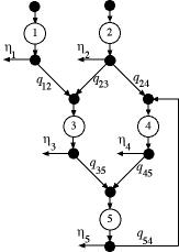
Figure 4 |
The pull network is illustrated in Fig. 4. For this structure
the flow through each operation may go to more than one operation,
and each operation may have several input flows from other operations.
This is a more general structure than the pull tree structure.
Flow is withdrawn or pulled from any of the operations. Again
we use
as the amount pulled from operation i. Indices are assigned
to the operations arbitrarily, however, it is often convenient
to assign the indices to be increasing in the direction of primary
product flow.
For the pull network we identify the proportion, ,
as the amount of the output of operation i required
for each unit of product passing through operation j.
The value of
may be any nonnegative amount to represent a variety of situations.
An assembly operation that requires one unit of each input to
be combined to produce one unit of a subassembly would have
the proportions equal to 1 for each input. A mixing operation
that combines inputs into a mixture would have input proportions
that sum to 1. An operation that requires more than one unit
of some input would be modeled with a proportion greater than
1 on the associated input.
The example shows an arc passing from operation 5 back to operation
4. In a practical instance, this might represent the reworking
of some part. Although we might be tempted to identify  as the proportion of the output of operation 5 returned to operation
4, this is not correct for a pull network.
is the proportion of the flow through operation 4 that comes
from operation 5. Similarly,
as the proportion of the output of operation 5 returned to operation
4, this is not correct for a pull network.
is the proportion of the flow through operation 4 that comes
from operation 5. Similarly,  is
the proportion of the flow through operation 4 that comes from
operation 2. is
the proportion of the flow through operation 4 that comes from
operation 2. |
| Push
Network
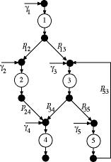
Figure 5 |
The push network is illustrated in Fig. 5. For this structure
the flow through each operation may go to more than one operation,
and each operation may have several input flows from other operations.
This is a more general structure than the push tree. Flow is inserted
or pushed into any of the operations. We use
as the amount pushed into operation i. Indices are assigned
to the operations arbitrarily, however, it is often convenient
to assign the indices to be increasing in the direction of primary
product flow.
For the push network we identify the proportion, ,
as the amount of the output of operation i that is
passed to operation j for each unit of product passing
through operation i. The value of
may be any nonnegative amount. Typically for a service system,
the sum of the proportions leaving an operation is equal to
1. This means that the flow is split among the several following
operations. It may be necessary to use other combinations of
proportions to represent different systems.
The example shows an arc passing from operation 5 back to operation
3. In a practical instance, this might represent the reworking
of some part.  as
the proportion of the output of operation 5 returned to operation
3. It is not necessary to define a proportion for the flow leaving
the system at operation 5. as
the proportion of the output of operation 5 returned to operation
3. It is not necessary to define a proportion for the flow leaving
the system at operation 5. |
| |

|
|