| |
Of course real inventory systems are not deterministic
as in the models considered previously. Although the models
that neglect uncertainly may yield results that are useful in
many contexts, it is possible to describe and analyze models
that explicitly include the uncertainty associated with some
aspects. There are many aspects that might be uncertain including
the lead time, the quantity that is actually received given
the amount ordered, or the amount demanded in any time interval.
It is impossible to provide analytical results for the most
general case. Here we consider only uncertainty in demand.
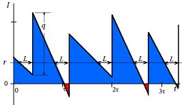
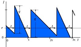
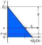
One possible stochastic inventory situation is
illustrated in the figure above. This is called the (q,
r) system and the add-in provides analysis and optimization
tools for this system. As for deterministic systems, the inventory
level is affected by demands and replenishments, but here we
show the demand process as variable, sometimes the demand rate
is high causing quickly declining inventory levels, while at
other times the demand rate is low with the inventory declining
more slowly. For this system, we have some inventory level r
at which we place an order for an inventory replenishment. This
is called the reorder point. The amount ordered is q,
the order quantity. After we place the order, we must wait for
some interval, L, the lead time, before the inventory
is replenished. Added to the models for the stochastic systems
are the risks and costs of shortages, shown as the red areas.
If the demand is high during the lead time (greater than r),
some customers will not be satisfied. We can set the reorder
point high to make shortages unlikely, but that will increase
the inventory levels, shown as the blue areas. The order quantity
affects both shortages and inventories as well as the cost of
replenishment. Our solutions will set system variables to balance
the costs of inventory, shortage and replenishment.In the following
we describe some of the options available for analysis.
The add-in allows stochastic
inventory models to be defined. The models allow the demand
during the lead time to be governed by a probability distribution.
All results are based on mathematical formulas that are described
in theoretical textbooks on inventory theory.
To create a model choose
Add Inventory from the menu. When shortages are allowed,
several options are presented for demand. The Deterministic
option creates the models considered previously. The other three
options define the probability distribution for demand during
the lead time. We describe the
options on the dialog below.
Infinite or Finite Replenishment Rate
| Infinite Rate
|
For the finite replenishment
rate, orders arrive in whole lots. The figure illustrates
the case where shortages are backordered. The inventory
level rises from its lowest level to an amount q
greater than the lowest level. The lead time (L)
and reorder point (r) are important for the (q,
r) system as the uncertainty of demand during the
lead time determines the cost of the system. If the lead
time were zero, the minimum inventory level would be zero
in each cycle and the maximum inventory would be q. |
| Finite Rate
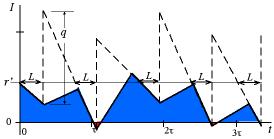
|
The same pattern of demand is shown at
the left for a finite rate system. This has the same shortages
as the infinite case as indicated by the equal time intervals
during which shortages occur. The average inventory and
backorder levels are reduced because replenishment amounts
arrive at a finite rate rather than an infinite rate.
Notice that the time intervals in which production is
actually taking place are equal. With a production rate
P, the interval is q/P. Since
the cycle times are not constant in the stochastic system,
the value of P must be great enough so that there
is a high probability that the complete lot is produced
before the next cycle starts. This is another penalty
associated with uncertainty. The production capacity must
have some excess to allow for the uncertainty in demand.
Our add-in requires that P >= D,
but does not enforce excess capacity.
Because the low points in inventory occur a little earlier
for the finite case than the infinite case, the reorder
point must be a little higher for the finite case than
the infinite case (r' > r). Because the approximations
used by the add-ins, this feature is not reflected in
the add-in results. |
Demand Probability Distribution
Poisson Distribution
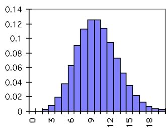
|
The uncertainty modeled is the demand during
the lead time. When the average demand per time interval
is D and the lead time is L, the average
demand during the lead time is DL. The Poisson
distribution is appropriate when demand events occur independently
and in single units. The parameter of the Poisson is its
mean value (DL). The standard deviation of the
Poisson is the square root of the mean. The figure shows
the Poisson distribution with a mean value of 10. Excel
has built-in functions to evaluate both the individual
probabilities and the cumulative distribution.
When the mean demand is greater than 30 it is difficult
to evaluate the Poisson probabilities accurately, so we
use the Normal distribution as an approximation. |
Normal Distribution
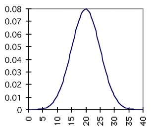
|
The normal distribution is a good approximation of
the Poisson for larger values of the mean. This option
uses a Normal distribution with mean DL. The
standard deviation is an input parameter. For some problems
it is interesting to vary the standard deviation to observe
the effects of uncertainty. If the Normal is to approximate
the Poisson, the standard deviation should set equal to
the square root of the mean.
It is convenient to have the parameters of the distribution
depend directly on the lead time. Then we can experiment
with different lead times without redefining the parameters.
Excel has built-in functions to evaluate the density
function and cumulative distribution of the Normal distribution. |
| Normal-LT |
For this option, the distribution of the demand during
the lead time does not explicitly depend on L.
Rather, both the mean and standard deviation are input parameters.
This is convenient for some problems, but in reality the
distribution of demand does depend on the lead time. |
Backorders or Lost Sales
 |
We have illustrated the backorder case in
the previous figures. In the figure we illustrate the lost
sales case. Here whenever a shortage occurs, the customer
is not served. When a replenishment arrives after a shortage
interval, the inventory rises to the level q because
there is no need to deliver backordered items. |
Shortage Cost
| Shortages Backordered
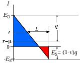
|
The figure shows an inventory
cycle assuming shortages are backordered. The cycle shows
the relevant expected values. Of course a sample cycle
will be different than shown because the demand during
the lead time may be less than r and no shortage
will be observed. In fact, the theoretical development
of stochastic inventories assume that shortages are rare
events. Some notation in the figure is defined below.
For the backorder case, we have three alternatives
for the cost experienced when a shortage occurs.
Cost per shortage event: Here there is an expense
in every cycle where a shortage occurs. The expected
shortage cost in a cycle is:
|
| Cost per unit short: Here there
is an expense for every unit that is demanded when
the inventory position is negative. The expected
shortage cost in a cycle is:
|
Cost per unit-time short: Here there is an expense
for every unit that is demanded when the inventory
position is negative. The expense is proportional
to the time spent in a backordered position. The
expected shortage cost in a cycle is:
|
|
Lost Sales
|
Cost per lost sales: Here there is an
expense for every unit that is demanded when on-hand inventory
is zero. A cycle of inventory appears in the figure with
expected values. The expected shortage cost in a cycle
is:
|
With stochastic models, additional parameters must be defined
as illustrated in the Parameters dialog below. The parameters
available depend on the options selected.
The parameters include the stochastic parameters that define
the probability distribution. For the Poisson distribution the
demand mean and standard deviation are entirely determined by
the expected demand during the lead time. For the Normal distribution,
the mean is the expected demand during the lead time, but we
specify the standard deviation. For the Normal LT option, we
specify the mean and standard deviation of the demand during
the lead time. The dialog above results if the Normal LT options
is chosen for on the inventory definition dialog.
One additional parameter is the Maximum Probability Short.
For stochastic models, the reorder point determines the risk
that the inventory will be exhausted during a cycle. Designers
often want to limit this to some small value. We provide this
option with this parameter. Optimum solutions are limited to
assure that this maximum is not exceeded.
The number of display options is also increased for a stochastic
model as shown below. The two options
on the bottom are only relevant when demand is random.
|