|
|
The examples for this section are in
the Teach IP demo workbook (teachipdem.xls). To solve
or change the model you must have the Teach IP add-in
loaded. Use the Relink buttons command to establish
links to the worksheet buttons.
|
Problem Definition
Begin the branch and bound exercise by clicking
on the Branch/Bound item on the Teach menu.
The program presents the problem definition dialog to accept
model data.
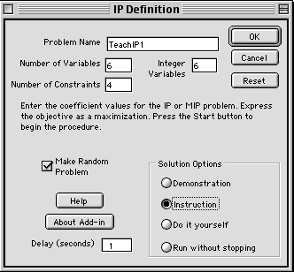
The program presents a possible name in the
Name field such as TeachIP1. There can be multiple
IP models in a workbook, and the integer number at the end
of the name will advance as IP models are added. The name
is used as prefix for a number of named ranges on the worksheet,
so once the name is specified it should not be changed. Names
must obey the Excel rules for naming ranges. The name should
begin with a letter, and include no spaces or punctuation
marks (a period is OK). The underline symbol may be used and
is often handy for two-part names such as P_1. A name like
P1 can't be used because it can be confused with a cell reference.
Fields are available for number of variables,
number of constraints and number of integer variables.
If the latter is fewer than the number of variables, the variables
with the smaller indices are assumed integer. The maximum
number of variables is 20 and the maximum number of constraints
is 10. The model must be expressed as a maximization. If the
Make Random Problem box is checked, the program will
provide random coefficients for the objective function and
constraints. Random problems have only less than or equal
to constraints. All coefficients are integer and positive.
A random problem will always have a feasible solution. When
the model is displayed the student can change any of the data.
One of four modes of operation is chosen with
a button in the Solution Options frame.
- Demonstration Option: In this mode, the program
takes the student through the steps of the procedure. Message
boxes describe the steps as they occur. The student presses
OK buttons to progress.
- Instruction Option: In this mode, the student makes
branching decisions and must tell the program when the current
incumbent is to be replaced and when an enumeration node
has been fathomed. A hint button is available that tells
the correct answers. Errors that would cause the algorithm
to go astray are not allowed.
- Do it Yourself Option: Here the hint button is
disabled and the student must make all the decisions directing
the algorithm.
- Run without Stopping Option: The program runs the
procedure with no student interaction. The approximate time
delay between steps is set in the Delay field. The
delay must be an integer number of seconds.
Except when the programming is running under the "without
stopping" option, the student is allowed to switch between
options.
Example Problem
The add-in builds the model structure shown below. Data has
already been entered for the example used for this section
(we use the same example as for the cutting plane approach).
Yellow ranges are controlled by the program or contain formulas.
These areas should not be changed by the student. In contrast
to the cutting plane approach, the branch and bound algorithm
does not require that the model coefficients be integer.
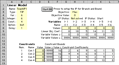
The format of the display follows that of other
mathematical programming add-ins in the collection. The model
is linear, and the linear objective coefficients of the variables
are placed in the range G9:L9. Simple lower bounds on the
variables are placed in the range G10:L10, and simple upper
bounds in the range G11:L11. The constraint information starts
in row 15. The range G15: L18 holds the linear constraint
coefficients. Each constraint has both lower and upper bounds.
The lower bounds are in the column range E15:E18, and the
upper bounds are in the column range F15:F18. The range D15:D18
holds the constraint values computed for the current solution.
The range in column B, B2:B8 holds information
required by the program and should not be changed by the student.
Starting the Procedure
Pressing the Start BB button creates the revised
tableau shown below. New rows are provided for the original
upper and lower bounds. This is necessary because the program
uses the simple lower and upper bound ranges to hold intermediate
bounds required by the branch and bound procedure. A new row
is also provided for the incumbent solution. As the algorithm
finds feasible integer solutions, the best solution is stored
in this range. There is also a cell for the incumbent objective
value. Initially there is no incumbent and the objective is
set to a large negative number. If a known integer solution
is initially available, it can be placed in this range.
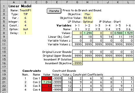
The solution to the first linear programming
relaxation is shown in the figure above. Colors are used to
emphasize features of the solution. The light green in the
variable value range indicates nonzero variables. Light green
in the constraint value range indicates loose constraints,
while red shows tight constraints. Not shown in this example
is the dark yellow that colors violated constraints.
The program constructs a representation of the
enumeration tree. The first vertex is shown in the figure
below. Each row describes a vertex of the tree. There are
seven columns in the display. The vertex at level 0 represents
the problem with no restrictions.
- Level: The number of tree vertices traversed from
the top of the tree to the vertex. Level 0 is the top of
the tree. This is also the number of simple bounding restrictions
placed on the LP.
- Vertex: The index of the tree vertex. Indices are
assigned in numerical order as the vertices are created.
- Variable: The branching variable at the vertex.
- Value: The upper or lower bound placed on the variable
at this level.
- Up/Down: The direction of branching, -1 for down
and +1 for up. Branching up implies that a simple
lower bound restriction is placed by this vertex. Branching
down adds a simple upper bound restriction.
- Visit: This is the number of times the vertex has
been visited. When first encountered the visit number is
1. When encountered through a backtrack step, the number
becomes 2.
- Relax: The value of the linear programming relaxation
including all the restrictions placed by vertices higher
in the tree. If the relaxation has no feasible solution,
the word Infeasible is placed in this field.

The Interaction
Begin by pressing the Iterate button
on the worksheet. At the top of the tree, there are no restrictions
on the variables. In this section, we are referring to the
LP solution in the figure above. We describe the example with
the dialogs that are used in the Instruction mode. When a
decision is required, the dialog is placed at the top of the
worksheet in a position that should not block the view of
important solution information. It can be moved if necessary.
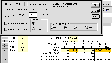
The dialog shows the objective values for the relaxation and
incumbent on the left. The student is to enter the index of
the branching variable in the Var. field.
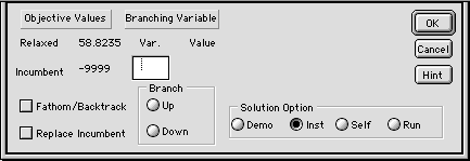
For the branch and bound procedure, the branching
variable is to be some variable that has a fractional value.
Pressing the Hint button on the dialog colors the fractional
variables yellow on the display. The index of the variable
with the largest fractional value is placed in the Var.
field. The fractional value is the difference between the
solution value and the nearest integer. For X6, the nearest
integer is 2 and the fractional value is 0.4706. Any of the
variables with fractional values can be used as the branching
variable, and the program will cycle through the options,
X2, X5 and X6, as the Hint button is repeatedly clicked.
The branching direction is either Up or Down as determined
by the button in the Branch frame.
Pressing the OK button makes the selection.
The Cancel button dismisses the dialog to return to
the worksheet. The Iterate button remains on the worksheet
so the student can resume the program. The student can change
the solution option by clicking on a different button in the
Solution Option frame.
The new LP solution is obtained after the program
has branched on variable X6 in the up direction. X6 previously
held a number between 1 and 2, but closer to 2., We branch
up by placing a lower bound on X6 of 2. Later in the
procedure we will branch down on X6 by placing an upper
bound on X6 of 1. The red field in the simple lower bound
range shows the decision.
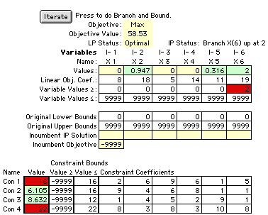
A new vertex, row 2 in the figure below, is
added to the tree. The visit number is set to 1 because this
is the first visit to this vertex. Observe that the added
restriction has decreased the value of the optimum LP solution.

Demonstration


