-Capacity Portfolio

We consider here a portfolio that consists of the machines used for processing in a manufacturing or service system. The system consists of several stations where processing takes place and where finished or intermediate products are withdrawn and sold. Sales cause flow through one or more stations. To handle that flow machines of fixed capacity must be purchased. Machines require investment and incur operating costs. One measure for the system is the profit which is the revenue from sales less the costs of manufacture. The model will include a constraint on minimum profit. The model will also include a budget constraint on the total initial investment. As the amount of flow increases through a fixed capacity machine, congestion grows in a nonlinear manner. This is best illustrated by the queues of a queuing network. We consider congestion in our model as the objective to be minimized. We build a nonlinear-integer mathematical programming model that considers congestion, profit and investment. The data for the problem is described on this page. The mathematical programming model is described on the next page. To create a model choose Capacity from the Portfolio menu.

The dialog below accepts the structural data for the system. Projects will provide capacity for stations that carry flow. The number of projects must be at least equal to the number of stations. The MARR is the minimum acceptable rate of return used for financial calculations. This must be expressed in terms of the time interval specified on the dialog, weeks in the example. The drive option, Push or Pull, is selected by the buttons on the right of the dialog.

In the following sections, we describe the various data items required by the analysis.

System Drive and Structure

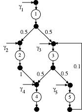
Pull Push	The drive and structure options for a system are also used for inventory analysis, process flow analysis and queuing networks. For more detail, please see these discussions. We provide here only a brief survey. The simplest pull and push systems have all stations arranged in a line as shown at the left. For a pull system, flow is pulled from the system at the station outputs. Flow pulled from station 5 passes through all the preceding stations. Although the figure shows output only at station 5, the models allow flow to be pulled from any station. Pull systems usually represent manufacturing systems where the products are sold after they are pulled. For a push system, flow is pushed into the system at the station inputs. Flow pushed into station 1 passes through all the following stations. Although the figure shows input only at station 1, the models allow flow to be pushed into any station. Push systems usually represent service systems where customers receive a variety of services after they enter the system.
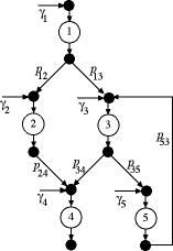
Push Network	More complicated systems are described as networks.The figure shows the push system used by the example. The structure of the system is described by the square transfer matrix P. For some applications the components of the matrix represent probabilities, but more generally the value is the flow passed to station j per unit of flow passing through station i. The value of may be any positive quantity and rows of the matrix need not sum to 1. The matrix used for the example is below. Note that the flow at station 1 is split to go to stations 2 and 3. The last row indicates that 10% of the flow leaving station 5 is returned to station 3 for reprocessing. Flow may enter at any station, but it is not necessary to define where the flow leaves. Given the entering flows, the flow in each station is determined by the solution of a set of equations involving P.
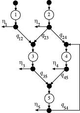
Pull Network	The figure at the left shows a pull system with 5 stations. The network structure of the pull system is described by the matrix Q. The component is the flow leaving node i per unit of flow passing through node j. Again the components of the matrix must be nonnegative. An example is provided by the matrix below. The columns of Q describe the inputs to a station. For example, column 5 indicates that for every unit passing through station 5, one unit must pass through each of stations 3 and 4. This is typical for an assembly station. For the pull system, the flows through all stations are governed by the flows pulled from the system. The solution of a set of linear equations involving Q determines the station flows.

The specification of either P or Q is part of the data for the Capacity Portfolio model.

After specifying the model parameters and selecting the drive option, the program constructs a math programming model based on a variety of data that must be entered on the forms provided on the worksheet. The data area is located immediately below the constraint area of the model. For the example, this is row 30 of the worksheet.

Three data items must be entered to describe the general features of the portfolio: the MARR (H31), the minimum value of the present worth (L32), and the amount of the budget available (L33). The dialog specifies the time interval as one week (Wk). The MARR is the minimum required rate of return per week. The value entered represents roughly 25% per year. We will have more to say about the time interval selection later. The other cells on the form below are filled by equations (H32, H33) or by algorithm computations (L31).

Project Data

Project data appears in the rows following the Portfolio data. There must be at least one project for each station. The data describing a project involves providing a single machine. Part of the problem is to determine the optimum number of machines.

A machine processes flow, and the data for one machine is shown in each column. Time dimensioned quantities are given in the time interval measure, week for the example. Each machine requires a investment expenditure at time 0 given in row 37. In every time interval during the machine's life there is an operating cost expenditure as given in row 38. Row 39 gives the salvage value of the machine at the end of its life. We have chosen 0 for all projects. The machine lives are specified in row 40. Since one week is the time interval for the example, the quantities in row 40 are in weeks. The financial quantities are combined using Excel financial functions to obtain a net cost per week in row 46. For a normal project the Investment, operating cost and salvage value are entered as positive numbers, although, investment and operating costs are cash outflows and the salvage value is a cash inflow.

The math program will select the number of machines of each type that optimizes the objective function. The minimum and maximum number of machines (servers for a queue station) are given in rows 41 and 42. The capacity, entered in row 43, is the amount flow that can be handled by a single machine at a station. For example, the N1 machine has a capacity of 37. If the flow through station 1 is greater than 37, certainly more than one of machine N1 must be provided.

The model will determine congestion with formulas from queuing theory. These formulas are based on the assumptions that the times between arrivals and the service times for stations are exponentially distributed. There are adjustments to these formulas when the service time variability is reduced. The Coefficient of Variation (COV) is the standard deviation of the service time divided by the mean service time. For exponential distributions the COV is 1, however, we provide the data item on row 44 to allow other values. Finally there is a component of operating cost that is linearly related to the flow through the machine. We call this the Processing Cost and enter values of the cost per unit in row 45.

Rows 47 and 48 hold values provided by the solution of the model. These values are 0 before the problem has been solved.

Station Data

The stations have data in columns H through L starting for the example in row 50. The unit profit in row 52 is unit sales revenue less raw materials cost. The sales volumes at the stations are variables in the model and the minimum and maximum sales are in rows 53 and 54. Recall that sales are pushed into station inputs for a push system, and sales are pulled from the outputs of the stations for pull systems. Rather than process the flow at the station, we allow the processing to be outsourced. The cost and WIP for outsourced units are in rows 55 and 56. Rows 57 and 58 report the results of the optimization and are initially 0.

Transfer Data

The transfer rates from one station to the next are given by the entries in P matrix starting at row 61. The example at the left is represented by matrix below. The Augmented Matrix is determined from the P matrix. The inverse of the augmented matrix is used by the model to compute the flow through the stations.

The model that uses this data is on the next page.