-Multiperiod Capital Budgeting

The multiperiod option creates a model similar to the capital budgeting problem but explicitly represents the individual time periods during a specified time horizon. Projects with non-uniform cash flows are easily represented on the data form. The most useful new feature is that cash flow demands can be specified for the individual periods and feasible portfolios must generate sufficient cash flows to provide for these requirements. 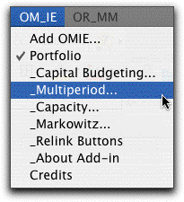To create a model choose Multiperiod from the Portfolio menu. We use an example adapted from class notes by A. Ruszczynski.

Three bonds are available to the investor. The cash flows for one unit of each bond are shown below. The negative number for year 0 is the initial investment and the positive numbers for the remainder of the years are the returns from the bond. All cash flows occur at the end of the year. Investment\Year 0 1 2 3 4 5 6 7 8 9 10 11 12 13 14 15 Bond 1 -980 0 60 60 60 60 1060 Bond 2 -970 0 65 65 65 65 65 65 65 65 65 65 1060 Bond 3 -1050 0 75 75 75 75 75 75 75 75 75 75 75 75 75 1075 Multiple units of each bond may be purchased from an investment budget of $250,000. Fractional amounts may be purchased. The portfolio must yield cash flows in the fifteen years as shown in the table below. The amounts are in $1000's. Cash is distributed at the end of each year. Year 1 2 3 4 5 6 7 8 9 10 11 12 13 14 15 Requirements 11 12 14 15 16 18 20 21 22 24 25 30 31 31 31 The investor is to select the number of units the bonds to meet the cash requirements and maximize the total cash available at the end of the last year (year 15). Cash not invested in the bonds earns a 5% return.

The Multiperiod menu item calls the dialog shown below. The number of projects is 3 to represent the three bond alternatives. The time horizon is 15. Excel financial functions used on the worksheet limit the time horizon to 28. We choose to maximize the final cash flow.

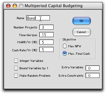
In addition to the MARR entry that is used to calculate net present worth values, we must include a rate for cash either not used by the initial investment or cash generated by the investments but not used immediately for cash requirements. We choose 5% for both quantities.

The Integer Variables checkbox and the Bound Variables checkbox are left unchecked for this example.

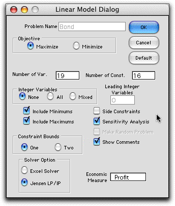
On clicking OK, the program calls the model formulation dialog from the Math Programming add-in.The fields have been automatically set to represent the problem. The experienced user may change the options on this dialog, but it is probably better to simply click the OK button. The dialog for the example is shown below. Although some of the data items do not appear to be correct, the add-in modifies some features after the model is created.

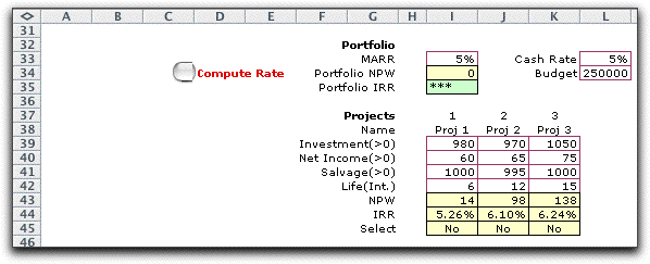
The form for the data describing the projects is placed below the math programming model. Although the returns for the example are not entirely uniform because of the zero returns for year 1, it is convenient to enter the data for the uniform cash flow in the range I39 through K42.

The math programming model is shown below after the solution has been obtained. The model is linear and continuous so its solution an be obtained with linear programming. The entries for variables 1, 2 and 3 (columns I, J and K) are automatically placed on the constraint form. We have replaced the cash flows in cells I16, J16 and K16 with 0's to reflect the non-uniform data. The requirements data is entered in column B. The budget amount is transferred by formula to cell B15. All the yellow cells contain formulas that link the data to the model, so generally they should not be changed. Non-uniform cash flows must be entered directly as constraint coefficients.

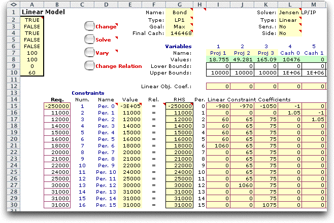
Only part of the model is shown. There is a variable for each cash flow over the horizon so the model proceeds to the right for 14 more cash flows. The only nonzero objective coefficient is for the cash flow for year 15. That coefficient is 1. The solution for the cash flows are below. The final cash flow value, $146,468, is provided by the optimum portfolio.

Clicking the Compute Rate button, shows the IRR for the optimum portfolio. The rates for the individual bonds are computed with Excel functions and shown in row 45. We have changed the formatting in the rate cells to provide additional decimal accuracy.

Parametric Analysis

It is interesting to perform a parametric analysis on the budget to see how it affects the final cash available and the mix between the bonds. We click the Vary button on the worksheet. This calls a macro from the Math Programming add-in that shows the dialog below.

We have changed the Vary Cell to L34, the cell that holds the budget amount. The default value of the Vary Cell is the right side of the first constraint, E15 for the example. Cell E15 holds a formula and the parametric analysis would replace the formula with numeric values. Varying cell L34 builds the table with the parametric analysis shown below.

As the budget declines, the objective function also declines. With smaller budgets, the mix of bonds favors the bonds with the shorter term. The amount of cash saved at time 0 also increases for the last three budget amounts. There is no feasible solution with a budget of $190,000.

Math Programming Model

The problem described above has an investment constraint plus constraints for each year in the time horizon. Separate variables are used to model the cash flow flow for each period.

The add-in allows several model variations. With the objective to maximize the net present worth of the portfolio and with the variables required to be integer, we obtain a model very similar to the Capital Budgeting problem. For the multiperiod model, however, the period cash flows need not be uniform and specific period cash requirements may be placed on the portfolio. The add-in allows extra variables and constraints to be included in the model. With these a variety of logical constraints can be imposed.

The NPW objective may not be appropriate when there are periodic withdrawals from the portfolio as assumed by this section. The capital budgeting problem assumes that cash generated by the projects either leaves the portfolio or remains in the portfolio but earns interest at the rate of the MARR. For the problem considered on this page, cash enters the portfolio at time 0 as the budget, leaves the portfolio with the scheduled withdrawals and finally leaves the portfolio at the end of the time horizon. Since the budget and withdrawals are fixed, their contribution to the net present worth does not depend on the decisions of the model. Only the final cash is affected. Thus maximizing the final cash is equivalent to maximizing the net present worth of the portfolio. This is not equivalent to maximizing the sum of the net present worth of the projects included in the portfolio.

Other Problems