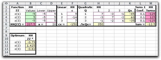
We use the example function below with constant, linear, quadratic and cubic terms.

The form describing the function is placed on the worksheet as shown. A similar form was described on the Add Function page. The optimum solution for the model excluding the cubic terms is determined analytically in the range A9:B14.

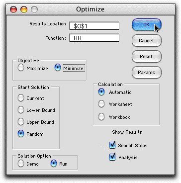
The Optimize dialog determines the direction (Maximize or Minimize) and starting point for the optimization. The Params button provides access to a number of parameters of the search process. These are described elsewhere with regard to the Teach NLP add-in. The Calculation option depends on the complexity of the model. For most cases the Automatic option is best. The program runs in either the Demo or Run mode. In the Demo mode the program stops at each iteration and provides an explanation of the process. To solve a problem in reasonable time, choose the Run mode. The Show Results boxes determine how much of the process is to be displayed on the worksheet. If neither box is clicked only the starting and ending solutions are shown.

For the example, we click the Minimize button to find a minimum point. The starting solution is randomly determined.

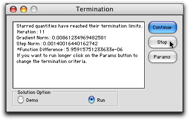
After a short time a termination message appears. Click Stop to see the results, Continue to go another iteration, or Params to change the termination criteria. For the example, the function changed very little in the final iteration, so the process terminated. The Gradient Norm is the norm of the gradient vector considering those variables not restricted by bounds. A value of 0 indicates an optimal solution. Here the gradient is small, but it is larger than the termination limit. The Step Norm shows the length of the last step. Again, it is small but it has not reached the termination limit.

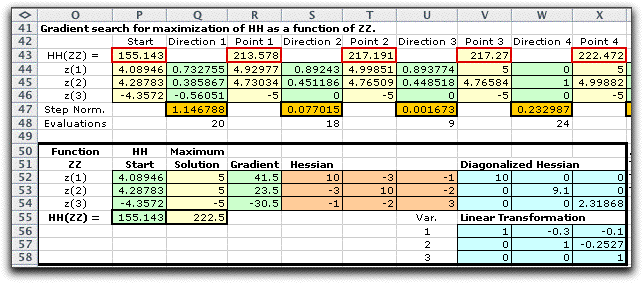
We show the first four iterations of the gradient search method below together with the analysis of the final solution.

Starting from a random point (Column P), the search process proceeds through a series of steps. At each step the gradient is estimated and used to set a search direction (Col. Q for the starting point). For a minimization the movement is in the direction of the negative gradient. The Step Norm in Col. Q is the length of the first step. The add-in uses a Golden Section method to find the length of the step. The Evaluations in Col. Q is the number of function evaluations required to evaluate the gradient and to make the first step. The process continues through a series of gradient evaluations and step moves until one of the termination criteria is met.

If the Analysis option is chosen, the add-in performs a second order analysis to determine the character of the function (convex, concave or neither) at the termination point. Based on the gradient and second derivative information at the point, the program makes its analysis. In the example case, the program indicates that the point is not a stationary point. We might observe, however, that the gradient is small and propose that the termination point is close to a local minimum. This is an interior minimum since none of the variables is on a boundary. The analysis process is discussed more fully on the Differentiation page.

Maximizing the Function

The optimization feature provided by this add-in is certainly limited when compared with capabilities of the Solver add-in provided with Excel. The optimization feature in the Functions add-in is applicable to problems for which the only constraints are simple lower and upper bounds. The Solver add-in and extensions that may be purchased from Frontline Systems are very general and useful in a wide variety of situations.

The features provided here complete to some extent the Jensen add-in collection with respect to optimization. The LP/IP Solver add-in and Network Solver add-in deal with linear optimization problems. The Optimization add-in and Combinatorial add-in deal with discrete problems. The Function add-in adds the optimization of continuous nonlinear models to the collection. This add-in can be easily called to solve other problems modeled by other collection add-ins. We can also control the optimization procedure in a manner not possible with the Solver add-in. The add-in is also helpful to those trying to teach or learn nonlinear programming.