|
|
|
|
Teach
Integer Programming Add-in
|
 |
|

| |
 |
The examples for this section are
in the Teach IP demo (teachipdem.xls). To solve
or change the model you must have the Teach IP add-in
loaded. Use the Relink buttons command to establish
links to the worksheet buttons.
|
Problem Definition
The cutting plane exercise starts when the student
clicks on the Cutting Planes item on the Teach
menu. The problem definition dialog is the same as for Branch
and Bound except that the Integer Variables field is
disabled. The cutting plane method described here only works
for pure integer problems. There is no need to specify the
number of integer variables, since it must be the same as
the number of variables.
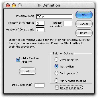
The program presents a possible name for the
problem in the Name field such as TeachIP1. There can
be multiple IP models in a workbook, and the integer number
at the end of the name will advance as IP models are added.
For the example problem we substitute the name Cut1 in the
name field. The name is used as prefix for a number of named
ranges on the worksheet, so once the name is specified it
should not be changed. Names must obey the Excel rules for
naming ranges. The name should begin with a letter, and include
no spaces or punctuation marks (a period is OK). The underline
symbol may be used and is often handy for two-part names such
as P_1. The name P1 won't work because it resembles a cell
reference.
Other fields specify the number of variables
and number of constraints. The maximum number of variables
is 20 and the maximum number of constraints is 10. The model
must be expressed as a maximization. If the Make Random
Problem box is checked, the program provides random coefficients
for the objective function and constraints. Random problems
have only less than or equal to constraints. All coefficients
are integer and positive. A random problem will always have
a feasible solution. When the model is displayed the student
can change any of the coefficients.
One of four modes of operation is chosen with
a button in the Solution Options frame.
- Demonstration Option: In this mode, the program
takes the student through the steps of the procedure. Message
boxes describe the steps as they occur. The student presses
OK buttons to progress.
- Instruction Option: In this mode, the student makes
decisions on which of the several cuts available is to be
added to the model. A Hint button is available which
indicates the possible selections. Errors that would cause
the algorithm to go astray are not allowed.
- Do it Yourself Option: Here the Hint button
is disabled and the student must make all the decisions
directing the algorithm.
- Run without Stopping Option: The program runs the
procedure with no student interaction. The approximate delay
between steps is set in the Delay field. The delay
must be an integer number of seconds.
Except when the programming is running under the "without
stopping" option, the student is allowed to switch between
options.
The button at the bottom of the dialog determines whether
loose cuts are deleted. As cuts are added, it may be that
previously added cut constraints become loose. There is no
guarantee that they will not become tight at a later iteration
of the procedure. An approximation is to delete cut constraints
as soon as they become loose. This reduces the size of the
model, but perhaps at the expense of more iterations. It is
even possible that the algorithm may never terminate when
this option is chosen.
Example Problem
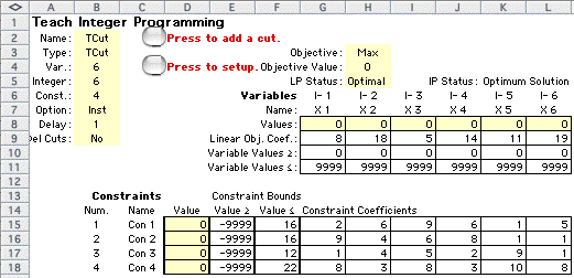
The add-in builds the model structure shown below. Data has
already been entered for the example used for this section
(we use the same example as for the branch and bound method).
Yellow ranges are controlled by the program or contain formulas.
These areas should not be changed by the student. In contrast
to the branch and bound approach, the cutting plane algorithm
requires that all constraint coefficients be integer.
|
| |
The format of the
display follows that of other mathematical programming add-ins
in the collection. The model is linear, and the linear objective
coefficients of the variables are placed in the range G9:L9.
Although ranges are provided for simple lower bounds (G10:L10)
and simple upper bounds (G11:L11), the default values or 0 and
9999 should not be changed. This implementation of the
cut procedure does not allow finite upper limits for the variables
(9999 represents infinity), and the algorithm assumes lower
bounds are 0.
The constraint information starts in row 15.
The range G15:L18 holds the linear constraint coefficients.
The constraint coefficients must be integer. Each constraint
has both lower and upper bounds. The lower bounds are in the
column range E15:E18, and the upper bounds are in the column
range F15:F18. The constraint bounds must also be integer for
this method. The range D15:D18 holds the constraint values computed
for the current solution.
The range in column B, B2:B8 holds information
required by the program and should not be changed by the student.
Starting the Procedure
Pressing on the Start Cut button solves the linear
programming (LP) relaxation of the integer problem, that is,
the integrality restrictions are dropped. As we will see, the
cutting plane procedure always solves the LP relaxation, however,
as the algorithm progresses new constraints are added, called
cuts. These cuts eliminate parts of the feasible region that
do not contain integer solutions. Finally, after a number of
cuts are added, we hope that the solution to the LP will be
integer. Some cut selections guarantee that an integer solution
will be reached, while others do not. We have observed that
some problems do not converge with this implementation even
though the theory says they should. When very many cuts are
added, the numerical inaccuracy of the LP solution procedure
may cause the process to fail.
|
 |
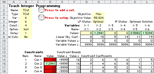
The solution to the first linear programming
relaxation is shown in the figure above. Colors are used to
emphasize features of the solution. The light green in the variable
value range indicates nonzero variables. Light green in the
constraint value range indicates loose constraints, while red
shows tight constraints. Violated constraints are indicated
by dark yellow in the constraint value range.
Gomory Cut
An area labeled Gomory Cuts is placed to the right of the constraint
display as shown below.

Gomory cuts are derived from the linear programming solution.
The procedure for deriving them is found in the textbook, so
we will not repeat it. We observe however, that the cuts involve
the nonbasic variables of the LP solution. The indices of the
nonbasic variables are placed above the yellow area in row 14.
To interpret the variable indices note that the original problem
has six structural variables. These are indexed 1 through 6.
The problem has four less than or equal to constraints. The
slack variables for the constraints are numbered successively
with indices greater than the structural variables. Thus the
slack variable indices for constraints Con1, Con2, Con3 and
Con4 are 7, 8, 9 and 10 respectively.
The procedure adds a single cut constraint at each iteration.
The cut will have a slack variable that is assigned the next
integer index. For example, the slack variable for the first
cut will be indexed 11.
A cut can be created for each basic variable of
of the model that does not have an integer value. In the case
of the example, the basic variables are X2, X5, X6, and X8 (SLK-2),
and all have fractional values, so four Gomory constraints are
shown in the display. The titles in column M indicate the basic
variable for which the constraint is defined.
The constraint at the bottom of the list is called a Dantzig
cut. We will describe that cut later, although we will not use
it in this example.
To illustrate the meaning of the table, consider cut C2. Row
C2 happens to be the simplex row whose basic variable is X8.
With the Gomory cut presentation as it is, it is difficult to
determine the basic variable that corresponds to each row. The
constraint in algebraic form with the constant on the right
is shown below.

|
| |
Every integer solution of the original
model must satisfy this constraint. Clearly, the current LP
solution violates the constraint because all the slack variables
are zero in the current solution. We will add this constraint
to the LP model and solve the problem again.
Before continuing the process we note that there are five valid
cut constraints available, the four Gomory cuts and one Dantzig
cut. We could in fact add one or all of them to the LP. We have
chosen in the implementation to add only one. There are several
heuristics to choose the cut to add. In these demonstrations,
the program uses the Gomory constraint with the greatest constant
value. For the example, this is C2.
The chosen Gomory cut can be added directly to the set of constraints
because it involves only structural or slack variables of the
problem. We go one step further however, and express the cut
entirely in terms of the original structural variables. This
is possible because very slack variable can be written as a
function of the structural variables. For the example, the constraints
C1, C3 and C4 are tight, so the slack variables for these constraints,
X7, X9, and X10, are nonbasic. To illustrate we write constraint
C1 with the slack variable X7 added to obtain the equality form.
In the second line the equation is solved for X7.

In a similar manner, each slack variable is expressed as a
function of the structural variables. These expressions are
then substituted for the slack variables in the Gomory cut.
The equivalents of the cut constraints are shown on the worksheet
to the right of the Gomory cuts. The figure below shows the
five cut constraints for the example.

Continuing the example we rewrite C2 in algebraic
form. We have multiplied the inequality by -1 to obtain positive
coefficients and we have placed the constant term on the right
side of the inequality.

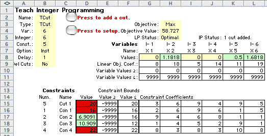
We add this constraint to the original problem.
The LP model with the new constraint is shown below. Note that
we add the cut to the top of the constraint matrix. We do this
to emphasize the cut constraints. As we progress, each new constraint
will be added to the top. The LP solution shows that the new
cut is indeed a tight constraint. The solution value is smaller
than the original relaxed objective function. This must be true
because the cut constraint makes the former solution infeasible.
|
| |
A little later on this page we present
the complete sequence of cut additions. As a preview, we show
the complete model after all cuts have been added. The procedure
adds seven Gomory cuts and the process finishes with the optimal
integer solution.
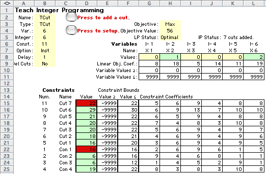
At the top of the worksheet in column P we have
a cell that will holds the number of cuts currently added to
the LP. In row 3 we keep a record of the objective function
as cuts are added. As the iterations progress, these will be
placed to the right of column P. The figure below shows the
objective values for all seven cuts. As expected the objective
value decreases as cuts are added.

At the bottom right of the worksheet we see the
list of Gomory cuts added during the procedure.
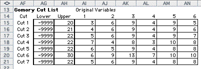
When we choose the option to delete loose cut
constraints, the final LP model is below.
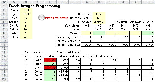
The final model includes only two cut constraints,
where seven cut constraints were present in the final LP model
when loose cut constraints were not deleted. The list of cuts
added is below.

Although 6 cuts were added, only two remain at
termination. The primary effect of deleting loose cuts is to
reduce the size of the LP model. |
| |
Dantzig Cut
The Dantzig cut is based on the requirement that at least one
of the slack variables must be a nonzero integer for an integer
solution to the original problem. This follows from the observation
that the current solution is not integer, so the sum of the
slacks must be nonzero. Since all constraints have integer coefficients,
the smallest nonzero value is 1. The Dantzig cut taken from
the first LP solution is written in algebraic form below. At
every iteration, a Dantzig cut will be formed by the sum of
the slack variables. The cuts will differ from iteration to
iteration because the set of slack variables changes.

Although it is has been shown that the procedure
will terminate with an optimum solution after a finite number
of Gomory cuts are added, there is no guarantee that the process
will terminate when only Dantzig cuts are added. |

|
