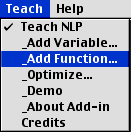
The second item on the Teach NLP menu presents the
function dialog shown below. A function has a location,
given by a cell address, and a name. The cell address
is determined by the cursor placement on the worksheet
when the dialog appears. The Function Location
text field is locked, so have the cursor placed at
the desired location when the menu item is selected.
A function definition may take up a number of cells
on the worksheet, so leave an appropriate amount of
empty space below and to the right of the cursor location.
The program gives a warning before the function overwrites
cells that contain information.
In the Function Name field, the program presents
one of nine preset names: F, G, H, J, K, L, M, N,
and O. When these names have all been used, the letters
are repeated, FF, GG, etc. When all the two letter
pairs are generated, three letters are used. The student
can change the suggested name. The name is used by
the program to identify various regions on the worksheet.
Every function depends on cells on the worksheet
that hold variable values. For this dialog, we expect
that a decision vector has been previously
defined using the Add Variable menu command.
The name of the variable range is placed in the Decision
Vector text box.
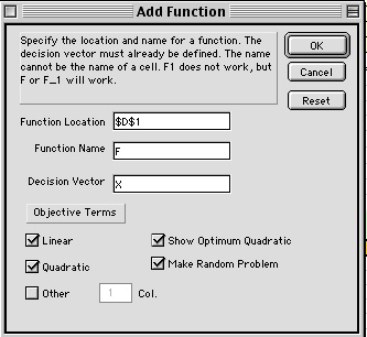
The check boxes in the lower half of
the dialog, determine the data structure that is placed
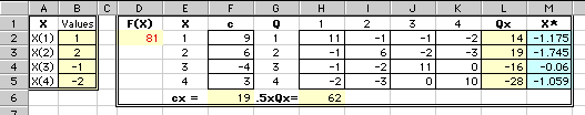
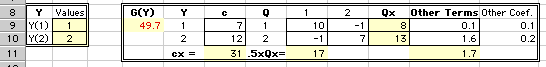
on the worksheet. The figure below shows the worksheet
areas created by the dialog. The range D1:L6 is first
cleared by the program. If cells in the range are
not empty, the program gives a warning. If the student
does not want the cells to be overwritten, he or she
can cancel construction of the function and choose
a new location.
The function name is placed at the top
left cell of the region and the Excel formula computing
the function is placed in the cell immediately below.
The cell with the red text is given the Excel name
that is the name of the function. In this case cell
D2 has the name F. The remainder of the range defines
data and results areas.
The second column, column E, names the
decision variable and provides indices for the linear
coefficient vector. The third column is for the linear
coefficients of the function. The values in the range
F2:F5 were assigned randomly for this case. They can
of course be changed. At the bottom of the column,
the matrix product cx is computed. Cell F6
is colored yellow to indicate that it contains a formula.
Although areas colored yellow may be changed by the
student, changes should be done very carefully.
Column G begins the presentation of
the Q matrix that holds the coefficients for
the quadratic terms of the function. The coefficients
are stored in the range H2:K5. Cell H6 holds the result
of the matrix computation:  ,
which is the contribution of the quadratic terms to
the objective function. The range L2:L5 holds the
results of the computation Qx. These results
are necessary for computing the number in H6. The
value in cell D2 is the sum of the linear and quadratic
computations. The value depends on the contents of
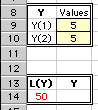
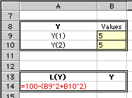
the decision variable X. The numbers in the variable
range B2:B5 are arbitrarily entered for this illustration.
,
which is the contribution of the quadratic terms to
the objective function. The range L2:L5 holds the
results of the computation Qx. These results
are necessary for computing the number in H6. The
value in cell D2 is the sum of the linear and quadratic
computations. The value depends on the contents of
the decision variable X. The numbers in the variable
range B2:B5 are arbitrarily entered for this illustration.