For the example problem, there are five possible causes for the computer failure, labeled: A, B, C, D and E. The first four are specific components of the computer, while E represents all other causes. In the following, we identify A through E as components. From past experience the repairwoman has probability estimates for each component. These are called the prior probabilities.

P(A) = 0.15, P(B) = 0.,2, P(C) = 0.3,

P(D) = 0.25, P(E) = 0.1.

In terms of Bayes' analysis, A through E represent the states of the world. The prior probabilities sum to 1, because we require that all possible states have been enumerated. We call the general prior probability P(y), where y is one of the states.

The decision problem would be much easier if the repairwoman knew the state. Then the appropriate component would be replaced and the expected cost of repair would be much reduced. The repairwoman can perform test X that will help identify the failed component. The test has three possible outcomes: x1, x2 and x3. Again through past experience she knows probabilities of the three test outcomes when a specific component is failed. These are called the conditional probabilities or the likelihood. They are given in the table below. The notation P(x|y) means the probability of outcome x given the state y.

These are not the probabilities necessary for decision analysis. To construct the tree we need the probabilities that the test will obtain each of the three outcomes, P(x). These are called the Marginal Probabilities. We also need the set of probabilities P(y|x), that is, the probability of state y, given the experimental outcome x. These are called the Posterior Probabilities. Both sets of probabilities are readily available from the application of Bayes' Rule, described in many introductory textbooks.

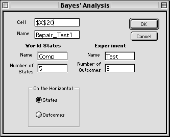
To construct the tables and do the computations for Bayes' analysis, we select the Bayes' item from the OR_MM menu. The dialog opens as below.

For the example problem, one of the five components has failed. A test, called Test1, will help identify the failed component. In the general terms of Bayes' analysis, we have five world states and three test outcomes. We identify the states with the abbreviation Comp and the test with the name Test.

The arrays that perform the Bayes' analysis can appear anywhere on the worksheet with its upper left corner at the cell shown at the field near the top of the dialog. The default cell is where the cursor lies when the dialog is presented, but it may be changed. Be sure that the arrays produced do not overwrite cells that contain data or formulas. A default name is provided when the dialog opens, but any legal Excel name may be used (no spaces or punctuation, starting with a letter). We make the practice of prefixing the name with the problem name so that names are not duplicated on different sheets of the workbook.

The arrays can be placed on the worksheet with either the states or outcomes on the horizontal as controlled by the buttons at the bottom. It is traditional to show the states on the horizontal, but when referencing the probabilities from worksheet cells it may be more convenient to place the outcomes on the horizontal. Both orientations are illustrated below.

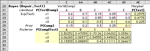
The figure shows the section of the worksheet showing the Bayes' analysis. As usual, yellow areas hold equations and should not be changed. All computations are accomplished with standard Excel formulas. The arrays with a white background and maroon borders are for data entry. The likelihood values, P(x|y), are entered in the cells starting at Z22. Note that it is not necessary to enter the values in the row for x3. The columns of the likelihood matrix must each sum to 1. We have assured this result by placing an equation in the row for x3 that computes 1 less the sum of the other two rows.

The prior probabilities are entered in row 25 for the example. It is unnecessary to provide an entry for E. It is computed by a formula so that the sum or the prior probabilities is equal to 1.

Of course, it is important that all probabilities entered be non-negative and no greater than 1.

Marginal Probabilities

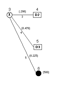
The marginal probabilities are computed in column AE for the example. They are used in the decision analysis for the probabilities on the arcs leaving node 3, the chance node representing the test X.

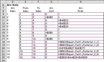
The figure below shows the formulas that are placed on the worksheet for this model. Rows 11, 12 and 13 of the worksheet model arcs 3, 4 and 5. The formulas point to the marginal probabilities in column AE of the Bayes' analysis. Note that we have used absolute references ($) so that if the arc array is sorted the references will not be disturbed.

The marginal probabilities could have also been referenced using the Excel INDEX function. The formula for cell H11 would be:

=INDEX(Repair_Test1_Marginal,1,1).

The marginal probabilities are given the name "Repair_Test1_Marginal" on the worksheet. The INDEX function picks the entry from this array in row 1 and column 1. The formula for cell H12 would select the entry from the second row.

=INDEX(Repair_Test1_Marginal,2,1)

The INDEX function is very useful when using named arrays. References are automatically absolute. Several other examples appear below for arcs that use the posterior probabilities. The name "Repair_Test1_Posterior" is assigned to this array.

Analysis with Outcomes Horizontal

The figure below shows the test outcomes on the horizontal. The results are all the same, but the numbers are transposed from the arrangement with the states on the horizontal.

Continued Testing

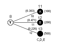
The example allows the repairwoman to perform two additional tests based on the result of experiment X. From the posterior probabilities we note that if test X has the outcome x1, the most likely source of the failure is component A or B. Test Y is now available. We assume that test Y can accurately identify the cause of failure if it is due to component A or B. If either of these indications are observed, the faulty component is repaired. Every other cause (C, D, or E) is grouped into a third category. If the test does not indicate A or B, the motherboard is replaced. Since test Y is perfect, the posterior probabilities for the failed component can be taken directly from row x1 in the posterior probabilities for test X. The results are shown on the figure at the left.

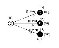
Similarly when test X indicates x2, the cause is most likely C or D. We can use test Z to accurately identify the fault if it is due to C or D. If the test does not indicate C or D, the fault must be in A, B or E. Rather than continue testing, the motherboard is replaced. The results of the tests together with the appropriate probabilities are shown at the left.