 |
With variables and functions defined, we
can proceed to find the values of the variables
that maximize or minimize the function.
This is the Optimize activity. While there
are many ways to optimize nonlinear functions,
we have only programmed two direct search
algorithms. These are only appropriate for
solving unconstrained problems. We expect
in later releases to have a greater variety
of optimization procedures, some applicable
to constrained problems.
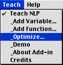
Both direct search methods are initiated
through the Optimize… menu item.
In this section we discuss the Gradient
Search method.
|
Optimize Dialog
Selecting the menu item presents the Optimize dialog illustrated
below. The top three fields are RefEdit fields. These allow
the user to specify ranges on the worksheet by selecting them
with the cursor. We prefer that the the student enter the
contents of these fields as described in this section, but
the RefEdit fields offer flexibility that will sometimes be
useful.
The top field on the dialog holds the address of the worksheet
cell where the results of the procedure will be presented.
Again, this is the cell at the top left corner of a range
that may extend considerably to the right and below the cell.
The program will issue a warning if parts of the worksheet
are to be overwritten. The default contents of the Results
Location field is the address of the current cursor location.
For this dialog, the field is not locked. A different address
can be entered manually, or the RefEdit field allows the user
to point to the desired location with the cursor.
The Objective Cell holds the name of the function
to be optimized. The Variable Range holds the name
of the decision variable. Of course, these names must have
previously been defined through the Add Function and
Add Variable menu items.
The remainder of the dialog holds various options.
The Objective frame determines the direction of optimization.
In addition to Maximize and Minimize, we include
the Evaluate button. With this option, the program
evaluates the point currently specified in the Y vector.
The Solution Method frame shows the two
methods currently available. In this section we are discussing
the Gradient direct search method. The Start Solution
frame indicates whether the procedure is to start from a zero
vector or from the current value of the Y vector. Two solution
options are provided. In the Demo option, the program stops
at each step with a description of the current activities
of the algorithm. This is useful for instruction. The Run
option goes through the steps of the algorithm without interruption.
The results presented by the program are determined
by the several check boxes on the dialog. They will be illustrated
through the examples on this page.
Search Parameters
The Params button allows the user to
specify stopping criteria and other parameters for the direct
search methods. Direct search algorithms for nonlinear programming
actually look for the optimum with intelligent trial and error.
There are no conditions that identify the optimum exactly,
rather we specify a set of termination criteria that indicate
that the program may be close to the optimum. Pressing the
Params button presents the dialog below.
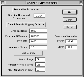
Here we define the various terms on the dialog.
Most of the entries on the dialog are stopping criteria for
the direct search procedure. Whenever the program reaches
a point that satisfies one of these criteria, it stops. If
the Termination Message option has been chosen, the
user can then change the criteria and allow the search process
to continue.
Derivative Estimation
- Step for Numerical Estimation of Derivatives: First
and second derivatives are estimated by finite difference
methods that compute the function for slightly different
values of the decision variables. This is difference between
successive values.
Direct Search Stopping Criteria
- Gradient Norm: The gradient is the vector of first
derivatives. It's norm is the magnitude of the gradient
vector. One expects this number to be small near the optimum.
When the gradient norm gets smaller than this limit, the
program stops and identifies the point as a stationary point.
- Function Difference: Near the optimum, the difference
between successive values of the objective function will
become small. When the difference is smaller than this number,
the program stops.
- Step Size: At each iteration of a direct search
method, a step is taken in some search direction that will
improve the objective function. Near the optimum, one expects
this step to become smaller and smaller. When the magnitude
of the step falls below the limit specified here, the program
stops.
- Number of Steps: At this number of steps, the program
will stop.
Line Search
- Search Range: The program uses a Golden Section
line search procedure to find the optimum point along a
search direction. The search direction is given by a vector.
The length of the step is the magnitude of the direction
vector multiplied by the number determined by the Golden
Section. This parameter is the maximum of the latter. In
cases where the direction vector is normalized, as for the
gradient search, the search range gives the length of the
maximum search step.
- Number of Evaluations: This is the number of steps
taken by the golden section method. The default value, 25,
gives a range of uncertainty at termination of around 10
raised to the -5 power. This is a very small number.
- Max Iterations at Limit: When the step size is
at the maximum step value 3 times in a row, the program
suspects that the optimum may be unbounded. The program
then stops.
Bounds on Variables
- When a component of the search vector goes outside the
range specified here, the program judges that the optimum
may be unbounded. The program warns the student and provides
an opportunity to terminate.
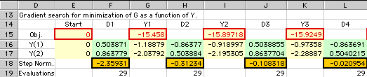
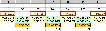
Direct Search with the Gradient Method
The OK button initiates the direct search procedure.
If the Search Steps output option has been chosen,
the progress of the search will be displayed as below. The
example is the G(Y) function defined earlier. The starting
point is the zero value of the decision vector. At each step
we see a yellow area showing the value of the objective function,
outlined in red, and the values of the decision variables.
The green areas show the direction vector, D(k). For the
gradient search, the search direction is proportional to the
gradient. For minimization the search goes in the negative
direction of the gradient, and for maximization the search
goes in the positive direction. We have normalized the gradient
vector so that its magnitude is 1. The yellow area below the
direction vector is the length of the step that minimizes
the objective function in the search direction. The number
below the yellow area is the number of function evaluations
necessary for the search. In this case the number is 29, the
number of iterations of the golden section search plus the
4 necessary to numerically estimate the gradient.
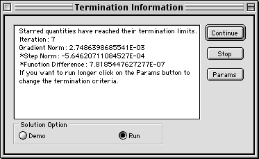
When the Termination Message box is checked,
the program stops when one of the stopping criteria is met.
The program presents a summary of the current results and
allows the user to change the criteria. In this case, we select
Stop and the final results are presented.
The extent of the results depends on the options
checked on the Optimization dialog. For the example, all the
options were chosen. The Row Titles option prints the
contents of column D. For some applications, we might what
a series of solutions for different problem parameters. For
a better presentation, show the titles only with the first
run. The Solution option shows the solution shown in
column E. The Gradient Option shows the gradient vector
for the variable values of the current solution. The Hessian
matrix is the matrix of second derivatives. With that option
chosen the program numerically estimates the Hessian matrix,
shown for the example in columns G and H. The Diagonalization
option, transforms the Hessian to obtain a diagonal matrix.
This matrix is used for the analysis.
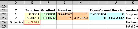
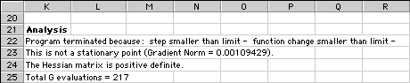
The Analysis option presents information about
the search process. The first line for the example shows the
termination mechanism. The second line shows the current magnitude
of the gradient vector. The value does not fall below the
limit of 0.001 specified in the parameter list, so the point
is judged to be not a stationary point. The diagonalization
is used to determine the character of the Hessian matrix.
In this case it is positive definite, indicating that the
function is convex at this point. For a stationary point this
would indicate a local minimum. Including the numerical estimates
of the gradient and Hessian matrices necessary for the final
analysis, the process required 217 evaluations of the G function.
This measure can be used to compare different search strategies.