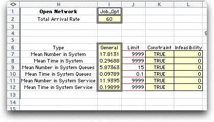
The Queuing add-in identifies cells for constraints immediately to the right of the system results. Column J holds the limit placed on the system result. Column K holds formulas indicating whether the result is less than or equal to the limit. Column L holds formulas computing the difference between the result and the limit. For a feasible solution all the cells in the range K7:K12 must be TRUE. The numbers shown below are for the initial values of the variables. The constraints are not satisfied for this solution.

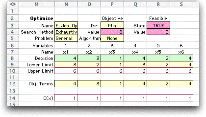
The Optimize add-in is automatically called to construct a combinatorial optimization form starting in column M. The cells colored green in row 8 hold the values of the decision variables, the numbers of servers in each of the six stations. Row 9 holds formulas that compute lower limits to the numbers of servers. There must be at least the number of servers at a station so that total service rate is greater than the total arrival rate. The upper limits (6) were specified in the dialog. These numbers may be changed after the form is constructed. Row 14 holds the unit costs of the servers at the stations. Since the example uses 1, we are minimizing the total number of servers used. Row 12 computes the server cost for each station. The sum of the yellow colored cells in row 12 is computed in cell P4. This is the objective function for the model. Cell R3 holds a logical expression that indicates whether all the constraints are satisfied (they are not for the initial solution). Cell R4 computes the amount of constraint violation. All formulas in the yellow or pink cells are created by the add-ins and no user interaction is required.

One additional important step is accomplished by the add-in. The numbers in the range N8:S8 are linked to the queuing model by placing formulas in the cells B5:G5. For example we see in cell B5 the formula:

=N8

The other cells are similarly linked. When the Optimize add-in manipulates the numbers in N8:S8, the server numbers in B5:G5 are changed. The functions in the queuing model compute the system results in column J indicating whether the solution is feasible. The variables are manipulated by the Optimize add-in and the worksheet computes the objective function and constraints.

To initiate optimization we choose Search from the menu. The dialog that defines the search strategy is shown below. There are many ways to search for the optimum. For illustration we choose Exhaustive Enumeration. This option will generate all values of the decision variables within the lower and upper bounds and evaluate the corresponding solutions. The add-in chooses the best feasible solution. This option guarantees optimality, but at the cost of many computations.

The add-in computes the number of evaluations required and presents the number in a dialog with the choice to continue or not.

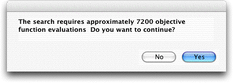
After some time, the algorithm finally finishes with the optimum solution shown below. The solution has 18 stations, which is the minimum number of stations that satisfies the constraints.

The system results for the optimum solution fall within the limits imposed. Individual station results are to the left of this display starting in column A. The demonstration file for this section has the complete worksheet.

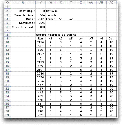
To the right of the combinatorial form is a summary of the time and number of runs required for the optimization. There is always one extra run because the optimum solution is repeated. The table below shows the 20 best solutions found. There is only one solution with 18 servers that satisfies the constraints, where there are several with 19 and 20.

Although exhaustive enumeration finds the best solution it takes a long time to find it. The approach is not practical for larger numbers of variables or greater variable ranges.

There are a number of heuristic alternatives that do not guarantee the optimum, but often give good results. The Greedy algorithm is a general procedure that changes the variables one at a time. Starting from an initial solution, the variable that improves the solution the most is increased of decreased by 1, and the process repeats. The process terminates when no change of a single variable improves the solution. We choose Greedy with the Search dialog.

For the example, the Greedy algorithm returned the optimum solution in 2 seconds on the author's computer.

Another option is random search that may be followed by an improvement process. The example below shows that 5 solutions are to be generated randomly. Each random solution is to be subjected to a 2-change procedure. The 2-change procedure selects pairs of variables and attempts to increase and/or decrease the variable values in an attempt to improve the solution. All pairs are considered and the process continues until no improvement is possible.

The results are below. Again the process finds the optimum. The runs are divided into Enumeration runs and Improvement runs. The enumeration runs are the five random solutions and the repeated optimum run. The improvement runs are due the 2-change method.

The Optimize add-in provides the capability for finding the best values of the parameters of the queuing system. Using the Optimize command of the Queue menu builds the model described here. Optimization with different objectives and constraints can be performed by using the Add Form command on the Optimize menu.