Return to Index
Operations Research Models and Methods
 
Computation Section
Queuing Add-in
 - Open Queuing Networks


The Queuing add-in computes values for the steady-state measures for a network of queues. The individual stations of the network may be either Poisson or non-Markovian. In the latter case the results are approximate. On this page we discuss open queuing networks where flow arrivals enter from outside the network and ultimately leave the network.

To add a model for a network of queues, place the cursor at the worksheet cell where the model is to be located and select Open Network from the menu. The dialog box below allows entry of the parameters of the model. Two arrangements are possible. The Serial arrangement assumes that stations are traversed by customers in sequence. Customers enter the system at the first station. After processing, they move the second station, and so on until the customer leaves the system after passing through the last station. The General option allows the flows to pass between stations in a very general way. We illustrate the Serial option first and later discuss the General option. Two options are also available for the distributions of interarrival times and service times. Clicking the Poisson button gives a model in which all times are exponentially distributed. The results provided by the model are accurate in this case. The General option allows non-Markovian stations in the network. When some stations are non-Markovian the results are approximate.

We illustrate the Poisson case first. When all arrival and service processes are Poisson, the resultant network is called a Jackson network. It has been shown that this kind of network can be analyzed by considering each station independently using the formulas for single Poisson queues. System steady-state results are accurately computed by adding the results for the stations.


The check boxes on the dialog determine optional presentation of the steady state results. The theory for the analysis of queueing networks does not allow finite queues or finite populations, so results related to these options are not available.

The Serial Case

Batch jobs submitted to a computer center pass through three steps: an input processor, the central processor, and an output printer. Jobs arrive to the computer center at random with an average rate of 10 per minute. To handle the load of jobs submitted, the computer center may have several of the three types of processors operating in parallel. The times for the three steps have exponential distributions with mean values as follows: input processor 10 seconds, central processor 3 seconds, and printer 70 seconds. When processors are not immediately available for a job, the job must wait in a queue. There is an unlimited queue for each processor. Our task is to find the minimum number of each type of processor and compute the average time required for a job to pass through the system.

The add-in constructs the arrays shown below to model the network with three stations. Data has already been filled in for the example problem. Note that the upper-left corner of the information is at cell B2, the location specified by the dialog. In columns C through E in row 2, we have replaced the computer generated names by the names for the three network devices. Row 3 shows the arrival rates. The yellow color in columns D through E indicates that these cells hold formulas. In fact, they all refer to the entry in cell G2, where the arrival rate to the first station of the network is specified. This cell is outlined in maroon to indicate that it may be changed by the user. Row 4 holds the service rates for the devices, which are computed from the mean processing times given in the problem statement. Row 5 holds the number of servers of each device. We have entered the minimum number of servers that can handle the load. Any smaller number results in an efficiency greater than 1 and an unstable system.


The remainder of the rows of the display show the results that are computed with the queueing functions provided by the add-in. The rows in columns C, D, and E describe the results for the individual stations. The station results are added together to obtain the system results in column G. For a network with arrivals and services governed by exponential distributions, each queueing station may be analyzed independently with the formulas derived for Poisson processes.

Reviewing the efficiencies for the three stations reveals that the central process is the least busy, while the printers are busy 97% of the time. Of the almost 50 jobs in the system, on the average, 43 of them are waiting or in process at the printers. From the system results we see that on the average a job spends about 5 minutes in the system.

Any number not colored yellow may be changed by the user to obtain new results. For example, one might wonder if increasing the number of printers would result in significantly lower throughput times for jobs. That can be immediately determined by increasing the number in cell E5.

The General Network

To illustrate the general network, we modify the problem slightly by changing the proportions of the jobs passing through each device.

All jobs must go through the input processor. Because of errors, only 80% of the jobs go through the central processor. Only 40% of the jobs passing through the central processor go to the output printer.

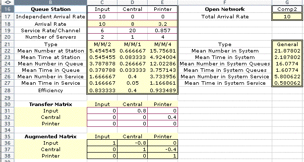
Since the different numbers of jobs pass through each device, we must use the General network option. The display for this option is shown below with the data entered for the computer problem. The display has been placed with its upper-left corner at cell B16.

For this option, a new data item appears in row 17, the Independent Arrival Rate. Each station may have arrivals from outside the system as indicated by the entries in this row. For the current example, all arrivals occur to the Input processor, so the other entries in this row are 0. The arrival rate in row 18 is a computed quantity and the contents of the row should not be changed. As before, the service rates and number of servers are controlled by the user. The numbers of servers shown here are the smallest numbers that will satisfy the demand at the three stations.

Data concerning the proportions of jobs passing from one station to another is entered in the table in the range C31:E33. We call this the transfer matrix because it shows the proportions of the flow transferred from one station to another. In row 31 we see that 80% of the flow transfers from the Input processor to the Central processor. The remaining 20% leaves the network. From row 32 we see that 40% of the flow passing through the Central processor goes to the printer.

The arrival rate shown in row 18 is computed with an equation involving the Inverse of the Augmented matrix. The Augmented matrix is the transfer matrix subtracted from the identity matrix The entries in the Transfer matrix are entirely general as long as the Inverse exists. An entry on the diagonal represents a recycling through the station. In many cases the numbers in the matrix represent proportions of flow transferred. A requirement of the Jackson network is that the routing be probabilistic. That is, a particular entity leaving a station will transfer the next with the given probability distribution.


The values for the mean number in the system, queue and service in column G are computed by summing the measures in columns C through E. The Mean Number entries represent the average number of jobs in the service, queue and system. The values associated with the mean time in the system, queue and service are determined by applying Little's Law using the Total Arrival rate in column G. The Mean Time entries often are not meaningful for individual jobs because the jobs follow different routes, but they do represent the average time considering all jobs.


Return to Top

tree roots

Operations Research Models and Methods
Internet
by Paul A. Jensen
Copyright 2004 - All rights reserved

Next Page