|
|
|
|
Teach
Dynamic Programming Add-in
|
 |
-
Build Your Own Model
|
|
|
The Dynamic Programming add-in provides the
structure on which the user can define a DP formulation. The
various model components are represented as Excel formulas
entered in the cells of the worksheet.
We use the knapsack problem is an instance of
a more general class of problems called Allocation of Scarce
Resources. We introduce the mathematical programming and dynamic
programming models for this class in this section. We use
the knapsack problem as an illustration of how the model is
implemented in Excel. By entering similar equations the student
can implement and solve any reasonably small discrete space
dynamic programing model.
|
|
|
Mathematical Programming
Model
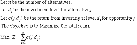
The problem is to determine the optimum investment level
in each of n alternatives. The return for each alternative
is given as a function of its index and the amount invested.
The objective is to determine an investment policy that maximizes
the total return. For the knapsack problem, the alternatives
are the collection of items from which a selection is to be
made. The level of investment for item j is the number
of the items to bring.
|
|
|
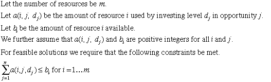
One or more resources are used up with the
decisions. In the case of the knapsack problem the single
constraint is the weight limitation.
|
|
|
The objective function and constraints comprise the mathematical
programming statement of the allocation of scarce resources
problem. Since the decisions are required to assume integer
values, neither linear nor nonlinear programming is an appropriate
solution technique. An enumerative solution procedure such
as integer programming or dynamic programming must be used.
Dynamic programming is very general with regard to the functional
form the objective terms and constraint terms. Linearity
is not required. Although most problems that can be solved
by dynamic programming can also be solved with integer programming,
the integer programming model will usually be quite large
and complex if nonlinear functions are part of the situation.
|
|
|
Dynamic Programming
Model
To formulate this problem for dynamic programming, a solution
must be described as a sequence of states and decisions.
The sequence of decisions is easily obtained by arbitrarily
ordering the investment opportunities. Thus the first decision
is the level of investment in opportunity 1, the second
decision is the level for opportunity 2 and so on. To complete
the model we must define each of the model components listed
below. Many variations in the problem statement can be accommodated
by minor variations in the model.
In the following we describe the mathematical formulation
of the model together with the Excel implementation. The
add-in constructs a number of named ranges on a worksheet
defining the model. All the ranges are prefixed with the
worksheet name, DP1_, for this example. This allows a workbook
to hold a number of dynamic programming models, each with
a unique name. In our descriptions we will use the prefix
DP1_ to explain the features of the model, however, that
prefix will differ for problems with other names.
|
|
|
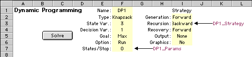
Options
The program is governed by a number of parameters that
identify the type, dimensions and optimization criterion
of the model, control the solution strategy, and specify
the material that is displayed during and after a run. The
program constructs two named ranges, DP1_Param and DP1_Strategy,
to hold this information. They are indicated in yellow in
the figure. The first four entries in the Params range are
set during the problem definition. The other entries in
the two arrays can be changed by choosing the Options menu
item from the Teach menu.
|
|
|
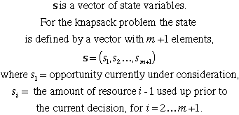
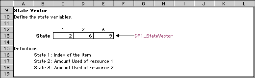
States
The dynamic process starts in an initial state. After each
decision the process moves to a different state. Finally
the process is finished when a final state is reached. The
state vector identifies the states of the process.
Mathematical Description
|
|
|
Excel Definition
The Excel model uses the worksheet region from row 9 to
row 19 to hold state information. The definitions of the
states are in rows 16 through 18. The number of rows will
expand to accept the number of state variables. The array
named DP1_StateVector is used during the solution process
to hold values of the state variables.
|
|
|
Decisions
Mathematical Description
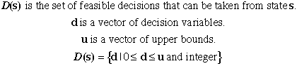
The vector of feasible decisions is defined by lower and
upper bounds on the decision variables. For the knapsack
problem, the decision is how many of an item to bring, so
the vector has only one component.
|
|
|
Excel Definition
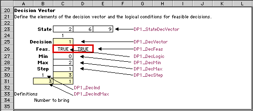
The decision vector and its bounds start at
row 20 of the worksheet. In row 23, we see the named range
DP1_StateDecVector. During computation this range will be
set equal to the values in the DP1_StateVector range defined
above. We do this because the feasibility conditions for
a decision might depend on the state definition. Formulas
implementing such a relationship can point to cells in the
DP1_StateDecVector range. Similar arrangements will be noted
for other components of the formulation.
The decision value is in row 25. If the decision
were a vector with more than one element, cells are provided
for each component. Below the decision value are cells for
the minimum, maximum and step size for each decision variable
(rows 27 through 29). During the solution process the decision
is taken through each possibility for every state. The limits
allow the values 0, 1, and 2 for the decision variable.
|
|
|
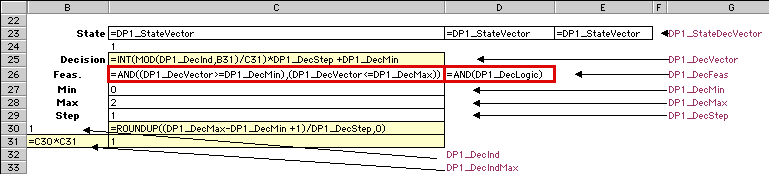
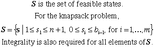
Excel Formulas
Row 26 holds equations that determine the feasibility of
the decision. Cell C26 contains a Boolean formula that returns
True if the first decision variable is between its bounds.
Cell D26 is true if all the decision variables are feasible.
The formulas that accomplish these computations are shown
in the Excel Formula view below. The formulas in both C26
and D26 use the AND Boolean function. In the latter case
the statement AND(DP1_DecLogic) is TRUE if all the cells
in the range DP1_DecLogic are TRUE.
We see in cells C23, C24, C25 the formulas that make these
cells equal to the cells in the DP1_StateVector range. These
formulas are added by the solution procedure, and need not
be a concern of the user.
Formulas in yellow cells are added by the computer when
necessary for the solution process. The formula in C25 accomplishes
the process of enumerating the set of decisions. The program
refers to DP1_DecInd, a number in cell B31. As that number
ranges from 0 to 3, the decision value in C25 ranges from
0 to 3. This isn't very exciting for this small case, but
the procedure is very powerful for enumerating all feasible
decisions for a decision vector with more than one variable.
The contents of cells C30, C31 and B31 are also used by
the program.
The important formulas for the user trying to implement
a different problem are those in C26 and D26. These can
be any Boolean functions or combinations of functions available
to Excel. Very complex feasibility conditions can be constructed.
|
|
|
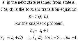
Forward Transition Equations
The forward transition equations compute the state that
is reached by taking decision d while in state s.
For the knapsack problem the decision moves to the next
opportunity and increases the amounts used of each resource
by an amount that depends on the decision.
Mathematical Description
|
|
|
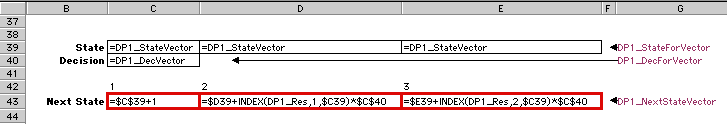
Excel Definition
We see below the Excel worksheet area implementing the
forward transition functions. The ranges DP1_StateForVector
and DP1_DecForVector copy the state and decision information
from the ranges in the upper part of the worksheet that
hold the state and decision vectors.
The range circled in red holds the next state. Although
in this case the program has filled this range with formulas
appropriate to the knapsack problem, the user can provide
his or her own formulas to implement any desired transition
functions.
|
|
|
Excel Formulas
The specific formulas for the knapsack problem are in row
43 in the figure below. The formula in C43 simply adds 1
to the contents of C39. C39 holds the index of the opportunity,
so cell C43 computes the index of the next opportunity.
Cells D43 and E43 compute the amount of resources for the
next state. The references to DP1_Res refers to the range
holding the resource usage amounts. The INDEX function is
helpful in that it chooses a number from a range for a given
row and column. Note that the unit resource is multiplied
by C40, and that cell holds the decision value.
Again, here is the place where the user will put new formulas
to describe the transition equations for different problems.
|
|
|
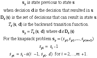
Backward Transition Equations
The backward transition equations are used to find the
previous state in a sequence of decisions. In this implementation
of the DP add-in we use these equations only for the recovery
of a solution after the Reaching procedure. If the Reaching
procedure is not used these functions can be left empty.
Mathematical Description
|
|
|
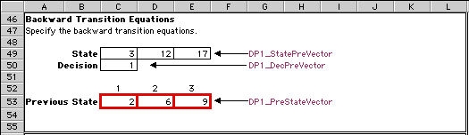
Excel Definition
The region implementing the backward transition functions
looks much like that of the forward transition functions.
In fact in many cases these functions are the inverse of
each others. If they are not procedure the Reaching procedure
will not work.
|
|
|
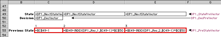
Excel Formulas
For the example the backward transition functions are implemented
in row 53. The previous state variable sp1, cell C53, is
simply one less than the state s1. The other functions reduce
the amounts of resources used and depend on the decision
vector.
|
|
|
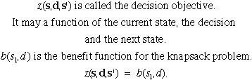
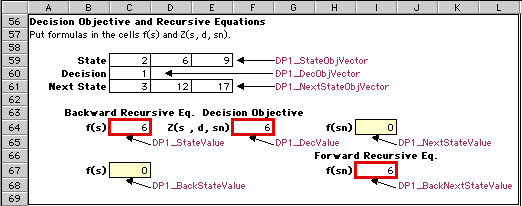
Decision Objective and Recursive Equations
Mathematical Description
These functions comprise the objective function of dynamic
programming. The contribution of a decision d taken
while in state s is computed by the decision objective.
This can be a function of s, d, and s'
(the next state reached).
|
|
|
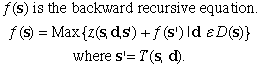
The backward recursive equation shows how the contribution
of a decision is combined with the results of the optimal
decisions starting from state s'. This is a recursive equation
because the value of f(s) depends on the value
of f(s').
|
|
|
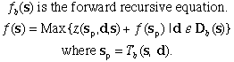
The forward recursive equation shows how the contribution
of a decision is combined with the results of the optimal
decisions made up to the previous state. This equation is
only used during the solution phase of the Reaching procedure.
If the Reaching procedure is not used, this function need
not be defined.
|
|
|
Excel Definition
The three quantities to be computed are scalar quantities
and are each computed in a single cell of the worksheet.
The decision objective in cell F64, the backward recursive
equation in cell C64 and the forward recursive equation
in cell I67.
|
|
|
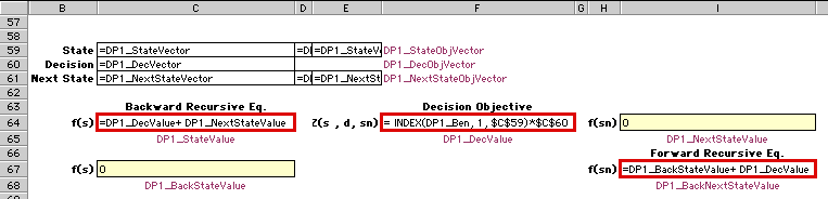
Excel Formulas
The decision objective for the example is in cell F64.
The unit benefits for the items are stored in DP1_Ben, and
the function multiplies the decision value times the unit
benefit.
The recursive equations are very simple in this case. The
Backward Recursive equation in C64 adds DP1_DecValue (cell
F64) to DP1_NextStateValue (cell I64). During the solution
process the computer puts appropriate values into DP1_NextStateValue
to solve the recursive equation.
In a similar manner the Forward Recursive Equation depends
on the cell DP1_BackStateValue. The computer controls the
content of this cell.
|
|
|
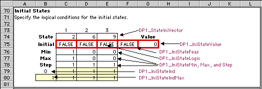
Initial States
The sequential decision problem can begin at one or more
initial states. When more than one is specified, the program
selects the one with the best objective.
Mathematical Description
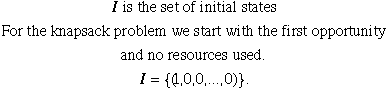
For the knapsack, we consider only one starting state (1,
0, 0). That is, we start with opportunity 1 and no resources
used.
|
|
|
Excel Definition
The structure on the worksheet allows a number of feasible
initial states to be defined. In the present case, because
the minimum and maximum limits are equal, only one state,
(1,0,0), is an initial state.
|
|
|
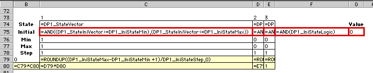
Excel Formulas
The important formulas in this case are those that determine
the Boolean value in cell F75. If this cell is True, the
state in row 74 is an initial state, while if the cell is
False the state is not an initial state. For this example,
the state is judged initial if its components lie within
the bounds.
|
|
|
Final States
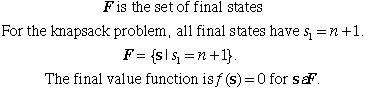
The decision process ends in a final state. Again, we use
sets to identify final states. For knapsack problem, a final
state has the first state variable equal to one greater
than the number of items.
Mathematical Description
|
|
|
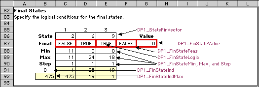
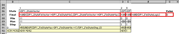
Excel Definition
The structure for Final states looks very much like that
for initial states. The state of cell F87 determines if
a given state (in row 86) is a final state.
|
|
|
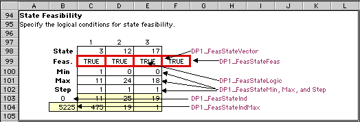
State Feasibility
Dynamic programming solution algorithms need only consider
states that will lead to feasible final states. Infeasible
states are those that do not. The definition of feasible
states is important because the number of computations in
a DP solution is important to the number of states considered.
If some states can be eliminated because they are infeasible,
computational effort will be reduced.
Mathematical Description
Although in general quite complex conditions can be used
to define feasible states, in the example we use simple
bounds. The validity of these bounds depend on the fact
that all the resource usage coefficients are nonnegative.
Excel Definition
The feasibility conditions start in row 94. They are very
similar to the structures for initial and final states,
except the minimum and maximum limits are different. In
addition to the primarily function of identifying feasible
states in the solution process, the structure below is used
by the exhaustive enumeration procedure for state generation.
When the DP1_FeasStateInd is assigned all the integer values
in the range 0 to 5225, all the states will have been generated.
Formulas placed in row 98 determine the state values from
the enumeration index.
|
|
|
Excel Formulas
|
|
|
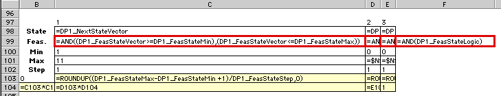
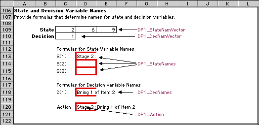
State and Decision Variable Names
Excel Definition
This area on the worksheet is not necessary for the DP
solution process, but it is very useful for presenting the
results of the DP solution in terms of actions. The cell
labeled DP1_Action is to hold a phrase that explains the
current state and decision. This cell is a concatenation
of the red bordered cells above. The latter cells have formulas
that generate string expressions.
|
|
|
Excel Formulas
|
|