|
|
|
|
Teach
Dynamic Programming Add-in
|
 |
-
Modeling with DP
|
|
|
 |
The examples for this section are in the
Teach DP demo (teachdpdem.xls). To solve
or change the model you must have the Teach
DP add-in loaded. Use the Relink buttons
command to establish links to the worksheet
buttons.
|
Problem Definition
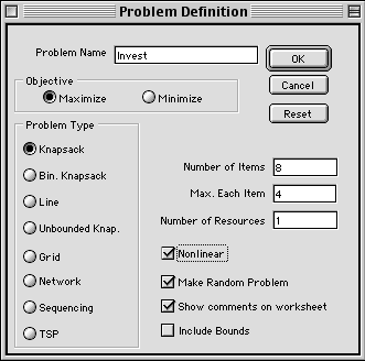
Selecting the Model option from
the menu presents the problem definition dialog
shown below. Fields accept the problem name and relevant
parameters. Clicking a button on the left selects
one of the problem types built into the program. After
entering data and pressing the OK button, a worksheet
is created with the name specified in the dialog.
Many ranges on the worksheet are given Excel names
with the preface being the worksheet name, so that
name should not be changed after the worksheet has
been constructed.
.
In the greater part of the worksheet
the program constructs the dynamic programming model
consisting of the state and decision definitions and
all of the other components listed in the text. We
delay describing those features until later in the
section and concentrate on the data structures for
the various problem types. When a button is pressed
to select a problem type, one of the buttons in the
Objective area is selected as the default direction
of optimization and the labels for the fields and
checkboxes on the middle right of the dialog box are
changed to reflect the problem type. The labels shown
are those used for the knapsack problem. The default
is to maximize the objective function. To change this,
simply click on the Minimize button.
The three checkboxes at the lower right
are common to all problem types. When checked, the
Make Random Problem box fills in the data form
with random numbers appropriate to the problem type.
Of course, these may be changed. The Show Comments
adds a small red label to some of the cells of the
worksheet. Clicking on a label presents a description
of the general purpose of the cell. The Include
Bounds button modifies the worksheet to accept
lower and upper bounds as described in Section 13.5
of the text.
Knapsack Problem
As shown in the dialog above,, the knapsack
model has three numerical parameters: the number of
items, the maximum number of each item that can be
packed, and the number of resource constraints. We
use the investment problem of Section 12.1 as an example.
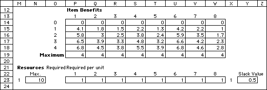
Pressing OK builds a data structure for the problem
as shown below. When the Nonlinear box is checked
a matrix of nonlinear item benefits is included on
the worksheet. Otherwise only one row is provided
for the linear return. Below the benefit area is a
row holding the maximum number of each item. In the
Resources area, a row is provided for each constraint.
|
|
Binary Knapsack
|
|
The dynamic programming model
for the binary knapsack problem is presented in
Table 6 and illustrated by Example 1 (references
are to Chapter 12 of the textbook). The option
automatically sets the maximum number of each
item to 1 and disables the second data field.
Of course the nonlinear option is not available
in this case. The data form constructed on the
worksheet is the same as for the linear knapsack
problem.
|
Line Partitioning Problem
|
|
Clicking the "line" button builds
a model for a 1-dimensional state space problem.
The dialog in the figure shows the settings for
the capacity expansion problem of Example 5. The
data form field requires the user to enter either
0, 1, or 2. The number entered is roughly equivalent
to the dimension of the data area set aside on
the worksheet. No data area is created if 0 is
entered. In this case, the user takes the responsibility
for creating a data area; alternatively, model
components may be computed with formulas not requiring
data.
|
|
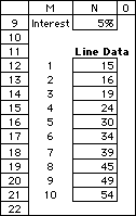
Capacity expansion costs
|
Entering a 1 in the data form
field creates a one-dimensional area on the worksheet.
The result is shown to the left, where the 1-dimensional
area is used to hold the expansion costs for the
capacity expansion problem. The interest rate
in cell N9 is the rate used for present worth
computations. This was placed on the worksheet
as an additional data item. One of the benefits
of using Excel is that data structures can be
constructed by the user to hold problem specific
information. Review of the workbook holding the
examples for this chapter will show many examples
of this.
The figure below illustrates the
use of a type 2 data form. The objective function
of the inventory problem of Example 6 has terms
that depend on the starting time and the number
of periods covered by a production run. The two-dimensional
form starting at cell N12 is partially shown in
the figure. It continues for 20 columns.
|
|
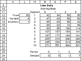
Segment costs for inventory problem
The entries in the cells are computed
with formulas described in Section 12.3. They
depend on the fixed, variable, and unit inventory
costs shown in Column L. The author of the worksheet
defined these cells. The formulas also require
the period demands given in row 24. Again the
user created and filled this data area. In general,
the program creates data structures that are typical
to the problem type. The user may add problem
specific parameters and coefficients.
|
Unbounded Knapsack
|
|
The unbounded knapsack problem
with one constraint has a single state variable
representation similar to a line problem. With
multiple constraints there are as many state variables
as resources. The dialog on the left asks for
the number of items and number of resources. The
data structures are like those for the bounded
knapsack problem except no maximum number range
is provided. The data is for Example 7.
|
Grid
|
|
The grid problem is described
in Section 12.5 and the data shown to the left
is for Example 8. The checkbox indicates whether
the model should include turn penalties. A problem
such as Example 8 requires two 2-dimensional matrices
to accept the data for both arcs directed vertically
and for arcs directed to the right. Data form
2 constructs these matrices. For data form 1,
1-dimensional arrays are created. These might
hold formulas or references to other data arrays
|
Network
|
|
This problem describes a general
shortest path network model on an acyclic graph,
as discussed in Section 12. 5. The dialog calls
for the construction of a network with 10 nodes
and 20 arcs. The arc data structure (Data Form
1) is a list of arcs each with an origin node,
a terminal node and a cost. The arcs are arbitrarily
ordered. When a 2 is entered in the Data Form
field 2, arc and node structures are constructed.
The arc structure is as for Data Form 1, but the
arcs must be listed in order of increasing origin
node. Each node is represented by a set of arcs
in a range of arc numbers. The node data structure
provides for the beginning and ending arc index
in the set identified for each node. Problems
entered using Data From 2 can be solved more quickly.
|
Sequence
|
|
Clicking the "sequence" button
creates a model for the single-machine sequencing
problem with tardiness penalties considered in
12.6. The data entered in the dialog is for Example
10. When the Data Form is set to 1, three 1-dimensional
arrays are created for job time, date due, and
unit penalty, respectively. When the Data Form
is 2, a 2-dimensional array is constructed with
job number identifying the row and number of days
late specifying the column. The Max Time determines
the number of columns. The matrix format allows
the imposition of nonlinear late penalties. When
the box at the lower left is checked, a matrix
is constructed to impose precedence ordering between
pairs of jobs. Such restrictions reduce the number
of states.
|
Traveling Salesman
|
|
The traveling salesman problem
considered in Section 12.6 corresponds to the
TSP button. The data, illustrated in the dialog
for Example 11, specifies the number of cities.
When the Data Form is 1, two 1-dimensional arrays
are created for the x and y coordinates
of the cities. When the Data Form is 2, a 2-dimensional
array is constructed to hold the costs (distances)
between all pairs of cities. The check box allows
for the construction of a matrix for the specification
of precedence ordering.
|
|
|
Excel Model
A DP model uses states and decisions to describe a
sequential decision process. A number of functional
expressions define the beginning, middle and end of
the process. A quantitative measure determines the costs
and/or benefits of the process.
When using this DP add-in for Excel, the expressions
describing the model must be placed into cells as Excel
equations. All DP model information is placed in first
few columns of the worksheet (the number of columns
depends on the number of state variables and decision
variables). Regions outside the model definition can
be used to hold problem specific data or equations.
We show below the Excel worksheet for the Knapsack
example. Areas colored light yellow hold equations or
data required by the program during the solution process
and should not be changed by the user. Ranges outlined
in red hold Excel equations that describe the decision
process. These equations can be entered by the user,
but in the case below they are filled by the computer
specifically to solve the knapsack problem. In the table
below, we provide a brief description of each of the
model areas. In the Build Your Own Model section,
the formulas are described in greater detail.
|
|

The data in the yellow areas describe features of the
model and the strategy for solution. The Solve
button initiates the DP solution process.
|
|
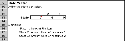
The state vector holds the values of the state variables
during the process. This area of the worksheet has no
equations but the state cells are varied by the computer
during the solution process. We have filled the state
with the values (2, 6, 9) to illustrate the equations
below.
|
|
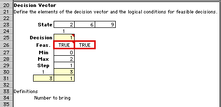
The decision vector holds the values of the decision
variables. We use the decision 1 (bring one of item
2) for illustration. In general, decisions are described
by a vector, but the knapsack problem has only one decision
variable.
The cells in row 26 hold equations that determine the
feasibility of a particular decision. In this case,
feasible decisions are within the range specified by
Min and Max (0 to 2).
|
|

The Forward Transition Equations describe how the situation
changes from one state to the next state when a decision
is made. In this case a decision to bring one unit of
item 2 results in a state change to (3, 12, 17).
|

The Backward Transition Equations move the decision
process in the reverse direction. We have filled in
the state (3, 12, 17). If the decision entering this
state was 1, the previous state must have been (2,
6, 9).
|
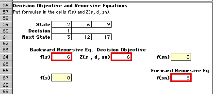
In this area we provide the benefit function for
a decision and the forward and backward recursive
equations used for the solution of the DP.
The decision benefit is the unit benefit for item
2 times the number of items (6*1=6).
We explain the recursive equations later.
|
|
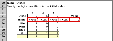
The process begins in an initial state. This region
contains the logical expressions that identify an initial
state. The given state (2, 6, 9) is not an initial state,
so we see the value False in the fourth cell
outlined in red.
For the example, the initial state must fall within
the Min and Max bounds. The only initial state is (1,
0, 0)
|
|
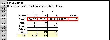
The process ends in a final state. This region contains
the logical expressions that identify a final state.
The given state (2, 6, 9) is not a final state, so we
see the value False in the fourth red square.
Again, the bounds determine the final state. In this
case, any feasible state with the first value equal
to 11 is a final state.
|
|
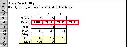
The process must pass only through feasible states.
This region contains, logical expressions that determine
state feasibility.
For the example, a feasible state falls within the
bounds specified by Min and Max. The specified state
is feasible.
|
|
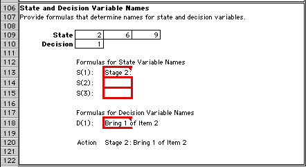
This region provides string expressions for states
and decisions. Expressions in the outlined cells construct
meaningful statements that define an action. These are
used in the presentation of the optimum solution.
|
|
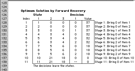
Pressing the Solve button initiates the DP solution
process. When it is complete, the output report above
is generated.
|
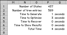
This summary at the top of the page
shows the number of states and tree entries and the
computation times for the parts of the solution process.
States are stored in a tree structure
that allows easy access to state information during
the solution process.
|
|
|

