Return to Index
Operations Research Models and Methods
 
Computation Section
Subunit Mathematical Programming
 Parametric Analysis

This section describes a recent addition to the Math Programming add-in. To obtain this feature, you must download a version of the add-in dated 6/14/04 or later.

Parametric analysis may be applied to any of the models constructed by the math programming add-in. A linear programming model with six variables and ten constraints is shown below. The data is random. The parametric analysis is performed by clicking the Vary button on the worksheet. Note that cell F15 is colored blue. For this example we vary the contents of this cell.

A dialog is presented for entering the data concerning the analysis. The Vary Cell is the address of a single cell on the worksheet. For the example we choose cell F15, however any cell whose value is relevant to the solution may be chosen. The example is the right-side value for the first constraint. The dollar signs in the cell reference are not necessary.
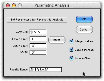
The next two fields hold the Lower and Upper limits on the range over which the parameter will vary. The Steps entry indicates the number of intervals into which the range will be divided. The Results Range specifies a range on the worksheet that will change with the parameter. The default value is the solution range, however, the range may be changed to show other values of interest. The range must be a single row or column of cells.

The check boxes at the right indicate respectively whether the parameter is to be restricted to integer values, whether the values will increase or decrease as the parameter is varied, and whether the add-in is to construct a chart of the objective function value as a function of the parameter.

The table below shows the results obtained when the right-side of the first constraint is varied. The first column (E) holds the parameter values. Note that the difference between adjacent values are not equal. This is due to the rounding necessary to obtain integer values. The second column (F) gives the objective function values for each parameter setting. The remaining columns (H through M) give the solution values. Nonzero values are highlighted in blue. For the example, we can clearly see that the linear programming basis changes as the parameter increases.
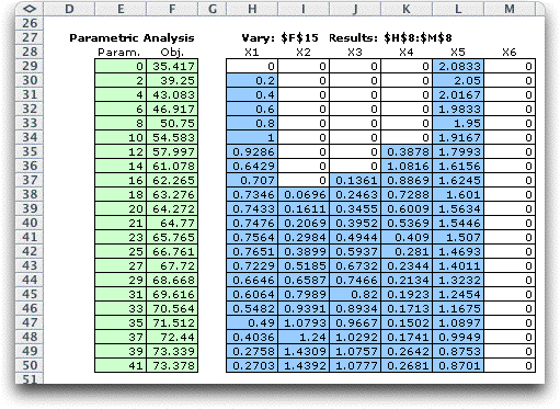
In the example we find a feasible solution for all parameter values within the range, but for nonlinear cases it is possible that there may be no feasible solution for some values of the parameter. Starting from the initial value (0 in this case), the program will solve the model. If no feasible solution is found, but the parameter increases until a feasible solution is found. Once a feasible solution is found, the parameter continues to change until an infeasible solution is again found. Then the process stops. Feasible solutions are shown, but values of the parameter that find no feasible solution are skipped.

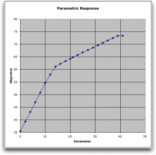
A chart showing the objective value as a function of the parameter value is constructed below the table. It should not be surprising that the curve is convex with respect to the parameter value.
 

Integer Programming

We solved the same model after requiring that all variables have integer values. Now a branch and bound procedure must be used to find the solution for each parameter value. Of course the process takes quite a bit longer. The tabular results are below.

The objective function chart shows the steps in the objective value caused by the discrete nature of the solutions.


Other Models


Parametric analysis is available for the other math programming models. For nonlinear models the Excel Solver must be used. For network and transportation models the Jensen Network Solver may be used. For network and transportation models the table of results and the corresponding chart are to the right of the data.

Nonlinear models may have trouble converging to a solution at every parameter value. When the first try at finding a feasible solution fails the program randomly generates a second initial solution. Hopefully the second try will find a feasible solution if one exists.

The parametric feature of the add-in is very general and can be used for a number of interesting problems. One possibility is to place the varying cell outside the model. Then several model features may be linked by Excel formula to the varying cell. The parametric analysis will affect many features of the model simultaneously.

The results range may too lay outside the model. For example perhaps only a few of the variables are of interest in a very large model. A row or column region of the worksheet can hold equations that link to the cells holding the important variables. Then, only these are shown in the results table. An example would be the integer variables in a large and complex mixed integer programming model.

If the Results Range box of the dialog is left empty, only the parameter and objective values are shown in the table.


Return to Top

tree roots

Operations Research Models and Methods
Internet
by Paul A. Jensen
Copyright 2004 - All rights reserved