Computation - Operations Research Models and Methods

Computation

Queuing Add-in

Adding a Queue

Queuing Results

User Functions

Non-Markovian Queues

Non-Markovian User Functions

Open Networks

Job Shop Example

Non-Markovian Networks

Closed Networks

Queue Simulation

Optimize

	Queuing Add-in
	- Queuing Results

The results display generated for the example case is shown below together with two other cases that demonstrate the effects of a finite queue and a finite population. The first six rows of the display give the parameters of the system and are not optional. Although functions cannot be entered directly into the dialog box, the parameters of the Queuing models can be replaced by formulas in the cells of the worksheet. This is useful for defining and analyzing networks of queues or modeling a system whose parameters depend on other calculations. The remaining rows show selected steady state results evaluated with formulas derived for Poisson systems.

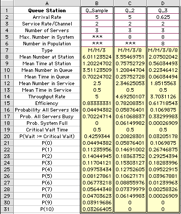
The column for Q_Sample provides answers to the questions originally posed. How many machines on the average will be waiting for repair? This is given by the mean number in the queue or 3.51. The mean number in service (or actually being repaired) is 2.50, so the total number in the system is 6.01. This is an interesting number because it represents the average inventory due to the maintenance operation.

How much time will a machine spend in the repair facility? This is given by the mean time in the system as 1.20 hours. The time dimensions are the same as those assumed for the arrival and service rates. The system time is broken into time in the queue (0.70 hours) and time in service (0.50) hours. These numbers are interesting because they describe the cycle time for the manufacturing process.

How often will the workers be idle? The efficiency result indicates that on the average the repair workers are busy 83.3% of the time. The state probabilities indicate that all three workers are idle simultaneously 4.5% of the time (P(0)), all three are busy 70% of the time (1 - P(0) - P(1) - P(2)), and the system is never full since in this case there is no limit to the length of the queue.

The columns for Q_2 and Q_3 show the results for systems with a finite queue and a finite population respectively. For the finite population case, Q_3, we have entered an arrival rate for an individual of the population as 0.625. When the system is empty, every member of the population arrives at this rate so the total arrival rate is 8*0.625 = 5. Thus, the third system is comparable to the other two, which also have arrival rates of 5.